
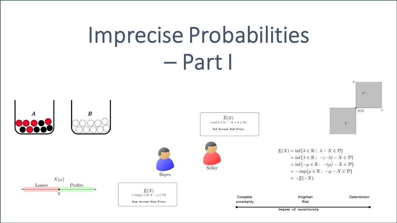
Introduction
The world is an uncertain place. How to measure and deal with uncertain quantities is an important problem for basically all branches of science, in particular, for measure theory, statistics, data science and finance.
The typical mathematical structure that is used nowadays is a probability space  . Thereby, the sample space
  is a given non-empty set and
  the (linear) expected value of a random variable
  with respect to the probability measure
  .
.
This mathematical model, however, requires strong assumptions that are quite often not fulfilled in real world. It is rare to find situations in which a probability measure fully reflects the corresponding real world situation. In finance, for instance, the normal distribution assumption is heavily used even though it is often not fulfilled.
Data can be scarce and human behavior might also be involved. In these cases, the uncertainty of the probability itself becomes a hard problem and using probability measures might not be sufficient anymore, for instance, due to the Ellsberg Paradox. In the theory of economics, this type of higher level uncertainty is known as Knightian uncertainty.
Example 1.1 (Ellsberg Paradox):
A person is shown two urns,  and
and  . Each of them containing 10 balls of red or black color. Urn contains 5 black and 5 red balls while there is no additional information about urn . That is, all balls in urn could be black or red or any combination in between.
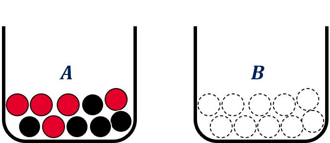 and each containing 10 balls whereby we do not know the distribution of the color red and black in urn
 One ball is drawn at random from each urn. The person is offered to make a bet on color of the ball chosen from either urn. Winning a bet the person receives, say, 1000 €. Possible bets are, for example, ‘the ball drawn from urn A is black’ denoted by  , ‘the ball drawn from urn is red’ denoted by
  , and, similarly
  and
and  . Let us assume that the person can pick one option for each of the following four bets:
- Bet on , or indifferent;
- Bet on , or indifferent;
- Bet on , or indifferent;
- Bet on , or indifferent;
We denote the corresponding probabilities of an occurrence of and by  and
and  , respectively. A similar notation is used for the occurrence of and . The probabilities of and as well as
  and
and  both each add up to
  given the additivity of the model.
It has been observed empirically that most subjects prefer any bet on urn A to a bet on urn  The decision that most subjects make with respect to the four bets is usually indifferent for 1. and 2., for 3. and for 4..
From the empirically suggested choice for bet 3. of drawing a red ball in urn , we infer  . Similarly, bet 4. implies
  and thus a contradiction.

There are several approaches to deal with uncertainty in a proper way, though. One way to deal with uncertainty is to use so-called capacities instead of probability measures .
In this post, however, we investigate so-called Imprecise Probabilities. The basic idea is to use a collection of probability measures (e.g. interval or set-valued probabilities), rather than a single (seemingly precise) distribution to model an uncertain event. Imprecise probabilities offer a framework for representing and reasoning about uncertainty in a more flexible and less seemingly precise manner than traditional probability theory.
We are going to focus on the theory put forward by Peter Walley [1]. However, this article is also based on [2] and [3]. Both are well-written and provide a good introduction and an overview on the topic of uncertainty.
Imprecise probabilities recognize that in many real-world situations, it’s difficult to assign precise numerical probabilities to events due to limited information or subjective uncertainty. Instead of a single precise probability value, imprecise probabilities use intervals, sets, or other structures to describe the range of possible probabilities.
We focus on the definition, basic properties and examples in the present Part I.
Part II is based on Part I and studies properties and structures of imprecise probabilities.
Overview
Let us assume that we are uncertain about the outcome of an event, that can be modeled using a set . The theory of imprecise probabilities is developed in terms of mathematical model  , whereby
- is a set of possible states of affairs of this event,
 is a class of –i.e. the set of all– gambles on which
- a real-valued set function
 , called lower prevision, is defined.
The so-called conjugate real-valued set function  , called upper prevision, can be derived via the relationship
  .
.
Hence, it is basically sufficient to focus just on lower or upper previsions.
is the set of possible outcomes, short possibility space, of a well-defined event, experiment, observations, occurrences, or any conceivable facts about the real world. In classical probability theory is the sample space.
A possibility space for the event is a finite or infinite set of elementary events  , i.e., mutually exclusive outcomes
  , that is exhaustive in the sense that other outcomes are deemed practically or pragmatically impossible. In classical probability theory, the possibility space is called sample space.
A gamble  is a bounded, real-valued function on , where
  can be interpreted as an uncertain reward or payoff whose value depends on the uncertain state . In classical probability theory, is called a random variable. The set of all gambles is denoted by
  .
.

A gamble is desirable for us, if we accept ownership of it when offered to us. Either as a bet that we buy or as a bet that we sell. Whether one is willing to accept a gamble depends on one’s belief in the outcome .
We model uncertainty about the event’s outcome (i.e. about the probability distribution of the possibilities) using a set of all desirable gambles  . That is, neither a single gamble nor its function values are uncertain. The uncertainty is reflected in a collection of different gambles instead of just considering one gamble.
Desirability Axioms & Function Vector Spaces
We equip the set of all gambles  with point-wise addition, point-wise scalar multiplication with real numbers
  , and the supremum norm (topology). Then, forms a normed real function vector space
  over , the bounded function (Banach) space to be precise.
Lower and upper previsions require commitments to act in certain rational ways, which is also reflected in the utility function of the decision-maker in the framework of imprecise probabilities.
As we know, a gamble is desirable for us, if we accept ownership of it when offered to us. We require the rationality criteria (D1) — (D4) as a logical consequence of the theory of upper and lower previsions.
Precise and Linear Subjective Utility Function
The key axiom (D1) and (D2) of the theory is that the utility for the outcome of a gamble is a linear function of the amount of the commodity that the individual gain from it. In other words, the personal utility function for the commodity is precise and linear. These assumptions are key since these requirements directly form a linear function vector space, in which we can model imprecise probabilities.
The theory of upper and lower previsions require commitments to act in certain rational ways. Let us first consider the following two out of four axioms.
(D1) If is desirable and  then
then  is desirable, i.e.,
(D2) If and  are each desirable then
  is desirable, i.e.,
Recall that the uncertainty about the event’s outcome is reflected in a set of desirable gambles  . By this, we split the set of all gambles into desirable and not desirable gambles
  . (D1) and (D2), in effect, require that the scale in which rewards
  are measured behaves like a linear utility scale and therefore inherits the vector space structure from . That is, the criteria of a linear subspace serve as axioms.
(D1) states that if you scale a desirable gamble with a positive real figure, it should still be desirable. So if you are offered a desirable gamble you should also accept each positive multiple of it.
Assume, we have two desirable gambles  , then
  is also accepted and thus considered desirable, i.e.,
  as stated in (D2).
Acccording to (D1) and (D2), a gamble’s desirability should be independent of the stake and the combination of two desirable gambles should also be desirable. In the context of imprecise probabilities, desirability is closely related to the idea of utility or value.
Avoiding Sure Loss and Accepting Sure Gain
The following questions (refer to [3]) are pivotal to the concept of desirability:
- Do we need to specify desirability for each gamble individually?
- Do we have to consider some specific sets of gambles to be desirable or not desirable?
- Can we argue that if some gambles are desirable, then other should be as well, i.e., can we automatically extend a partial specification?
The answer to the last question 3. is obvious given the result from last section about the vector space structure of . The linear hull of each  also has to be desirable. The answer to 1. is therefore ‘no’.
Are there compelling reasons to insist that some gambles should be desirable or not desirable, independent of the information available to us about the event’s outcome?
And indeed there are:
Any gamble that gives a positive payoff or reward without ever giving a negative one needs to be considered desirable in this setting. In addition, any gamble that gives a negative payoff or reward without ever giving a positive one needs to be considered not desirable.
These two criteria can be formalized as follows:
(P1) Accepting partial loss
If  then
then  or
or 
(P2) Accepting partial gain
If  then
then  or
or 
Note that means that for all  the function value is always greater than zero. Thereby,
  can also be interpreted as the zero gamble, where you get for every possibility .
That is, you are certain about the gains and losses and thus certain about the final payoff as sketched in the following graph. No matter which is going to realize, we already know that the outcome will be positive and thus the function value lies in quadrant I. A toy illustration is shown in Fig. 2 below.

Fig. 2: Sketch of a function vector space with a two-element possibility space  . The highlighted quadrants I and III reflect the possible function values
  and
and 
We see that the so-called positive orthant  and negative orthant
  must, respectively, be included in and excluded from the set .
In addition,  and
and  is not a vector (sub-)space since the additive inverse is not an element of and , respectively.
Let us now slightly relax the requirements made in (P1) and (P2) and assume you are offered a gamble, where you are either guaranteed to
- experience a loss regardless of the decision you made, i.e.,
 or
or 
- experience a gain regardless of the decision you made, i.e.,
 or
or  .
.
Note that  is the interior of a set.
This effectively means that there is no uncertainty about the fact that the decision will result in either a loss or a gain. The theory of lower and upper previsions requires that such gambles where you are sure about a loss are not considered to be desirable. Likewise, gambles where you are sure about a gain are considered to be desirable. Let us formalize these rationality criteria according to the theory of lower and upper previsions in the following axioms.
(D3) Avoiding sure loss
If  then is not desirable.
(D4) Accepting sure gain
If  then is desirable.
Lower and Upper Previsions
The theory of imprecise probabilities consider gambles, whose possible outcomes are gains or losses of a single commodity.
Lower and upper previsions generalize probabilities and expectations we usually encounter in the classical probability theory, though this theory falls squarely within the subjective approach of probability.
Subjective means in this context behavioral, that is, a subject’s probability (i.e. belief) for an event reflects his willingness to take certain actions whose outcome depends on its occurrence, such as accepting bets on or bets against the event at certain betting rates.
The outcome of a gamble is uncertain and depends on the events of interest as well as on the utility function of the individual decision-maker. Recall that a gamble  is a bounded real-valued map on the possibility space. It represents an uncertain reward, whose value is if the outcome of the experiment is . This reward is expressed in units of some linear utility scale as outlined in the section before.
The theory of lower previsions considers two types of transactions involving a gamble :
- Accepting to buy for a price
 , which comes down to accepting the gamble
- Accepting to sell for a price , which comes down to accepting the gamble

Note that  is the buying or ask price that we receive as a seller while
  is the selling or bid price we need to pay as a buyer. Inflows and outflows relative to a certain party are represented by positive and negative signs, respectively.
Let us now assume that a bet has been accepted by both parties of the deal, i.e. by the seller and the buyer. This implies that a price  is acceptable for both, i.e., the corresponding bid-ask spread is zero. Figure 3 illustrates the payoffs for both parties in this case. Note that can be positive and negative.

Fig. 3: Exchange of cash flows to the buyer and seller. The payoff of the gamble depends on the event that realizes and might be positive or negative for the buyer. That is, the outcome of is uncertain
We denote  for the infimum (greatest lower bound) and
  for the supremum (least upper bound). Both
  as well as
  are finite since a gamble is bounded by definition. We write
  if
if  for all .
A subject’s lower prevision  for a gamble represents his supremum acceptable buying or ask price for , which is the highest price
  such that the subject accepts to buy for all prices
  . In other words
(1) 
where is the set of gambles that our subject finds desirable. (1) implies that the subject is willing to pay  for the uncertain reward , or in other words, that the transaction
  is desirable for the subject for every
  . Nothing is said about whether the subject would actually buy the gamble for the price given the definition of the supremum.
We can also consider our subject’s upper prevision, or infimum acceptable selling or bid price, for the gamble , which we denote by  . It is the lowest price
  such that the subject accepts to sell for all prices
  . In other words
(2) 
(2) implies that the subject is willing to sell the gamble for  . That is, the transaction
  is desirable for the subject for every . Again, nothing is said about the price itself.

Fig. 5: Illustration of upper and lower prevision of a buyer and a seller
The following Fig. 6 illustrates the general interrelation between the lower and upper prevision focused on the payoff function compared to the situation as shown in Fig. 5.

Fig. 6: Interrelation between the lower and upper prevision in the general case, i.e. when the lower prevision does not necessarily meet the upper prevision.
Note that a fair (market) price exists if lower and upper prevision meet. In this case no ‘undecided’ interval exists.
Let us apply the theory in the next example.
Example 4.1 (Urn, modified version taken from [1]):
Suppose a ball is drawn from an urn with red, white and black balls. We are offered a reward depending on the color of the ball:
- We get €10 if red ball is drawn,
- we get €5 if a white ball is drawn, and
- we get €0 if a black ball is drawn.
The corresponding gamble is based on the possibility space  , where
  ,
,  and
and  stands for ‘black’, ‘red’ and ‘white’, respectively. That is, is defined by

The bet is desirable since all payoffs are not negative. In addition, we might be willing to pay some fixed amount of money, say  €, in order to buy the gamble and thus to receive the uncertain reward. We are going to suppress the € symbol in the rest of this example.
The increase in wealth for the buyer would be  . That is,
  if a red ball is drawn,
  if a white ball is drawn, and
  if a black ball is drawn.
The supremum amount of money , we are willing to pay to buy the gamble, will be our lower prevision for the gamble .
If, for instance, we are absolutely certain that there is no black ball in the urn, we should be disposed to pay up to  since this is the least we will get given the subject’s belief. In other words, the wealth will not be decreased no matter what event –i.e. a red or a white ball is drawn– will arise. Hence, the subject will assume some sort of worst case given its belief.
If, for instance, the subject is sure that only red balls are in the urn, then we the buyer should pay less than 10 since +10 is the worst payoff the buyer can have given his belief.
On the other hand, we could also consider selling the gamble for a fixed price  . Our increase in wealth will then be
  if the red ball is drawn,
  if the white ball is drawn, and if the black ball is drawn. The infimum amount of money , that we require in order to sell , will be his upper prevision .
If, for instance, the seller is absolutely certain that there are only red and white balls in the urn, he should accept to sell for any price  . Apparently,
  is the worst payoff the seller can have in the gamble under this condition.
The last example demonstrated that the price, that a rational buyer is willing to pay and a rational seller is willing to sell for this gamble, respectively, depends on the presumed distribution of the white, red and black balls in the urn.
If we generalize that observation, we can see that the prize of a gamble directly depends on probabilities assigned to the possibilities .
If  on with possibility set is a lower prevision, the conjugate upper prevision
  is defined on the domain
  by
by  . A benefit under a lower is going to be a loss under an upper prevision. Note that may be defined on a different domain from .
In the theory of lower and upper previsions, we are not paying attention to the subject’s entire set of desirable gambles but rather try to model our subject’s belief by looking directly at this lower and upper previsions for a number of gambles.
Recall that we model uncertainty about an event’s outcome (i.e. about the probability distribution of the possibilities) using a set of all desirable gambles of a subject. Suppose our subject assesses lower previsions for all gambles on some subset  . This defines a real functional
  , which is the lower prevision with domain . There is an analog definition for the upper prevision with domain
  .
.
Since selling a gamble for a price  is the same thing as buying the gamble
  for the price
  , buyer and seller need to be disposed to accept these transactions under the same conditions. Hence, the seller’s infimum acceptable selling price need to agree with the buyer’s supremum acceptable buying price for . Again, in this case the bid-ask-spread is zero, i.e.
  as illustrated in Fig. 4:

As a consequence, given the lower prevision on a set of gambles , we can define the so-called conjugate upper prevision on  , by
, by  , and vice versa. Taking this into account, as we can freely go from one concept to the other, it suffices to discuss only one of them.
Without loss of generality, we are going to focus on lower previsions or to put it differently on the buying side.
Coherent Sets of Desirable Gambles
The axioms (D1) – (D4) are fundamental for the theory of imprecise probabilities. The first two axioms (D1) and (D2) basically require that the set , that contains all desirable gambles, is a (function) vector space.
What about (D3) and (D4)?
Let us consider axiom (D3) closer. Let be the buying price for the gamble . If  is negative no matter what outcome is going to be, then needs to be a non-desirable gamble.
Hence, from a buyer perspective a desirable gamble needs to fulfill the condition
(3) 
If  for all , then it’s going to be a sure overall loss for the buyer. This needs to be avoided according to axiom (D3), such that the difference of both need to be positive for some .
The in-equation (3) requires that the overall payoff  is at least of positive utility for some . Hence, it is sufficient in (3) to check the best case(s), i.e. to take the supremum over .
If we apply the additivity axiom (D2) to a finite set of desirable gambles  with
with  and
and  , it follows that
(4) ![\begin{align*} \sup_{\omega\in \Omega}\ \{ \sum_{i=1}^{n} \left[ X(\omega) - \underline{E}( X(\omega) ) \right] \} \ \geq 0. \end{align*}](https://www.deep-mind.org/wp-content/ql-cache/quicklatex.com-5dd92122830180c2dfa5d148be418150_l3.png "Rendered by QuickLaTeX.com")
To motivate condition (4), assume that it is not satisfied. Then there are  ,
,  in , and
  such that
![\begin{align*} \sum_{i=1}^{n}{ \left[ X_i - \underline{E}(X_i) +\epsilon \right] } \leq -\epsilon, \end{align*}](https://www.deep-mind.org/wp-content/ql-cache/quicklatex.com-ca61bed43515b032d0121df133016818_l3.png "Rendered by QuickLaTeX.com")
meaning that the sum of the desirable gambles  results in a loss of at least
  , no matter the outcome of the event . Since the sum needs to be desirable by (D3), this violates (D1). Contradiction.
Let us try to illustrate that in an example.
Example 5.1 (Urn continued)
A subject is faced with the bet as outlined in Example 4.1:

The subject is absolutely certain that there is no black ball in the urn, such that he is disposed to pay up to since this is the least he will get given his belief. Therefore, he is avoiding a sure loss for the gamble based on his belief.
Another gamble , defined by

, is also offered to this subject. Let us assume the subject is willing to pay 6 for the bet , then the overall payoff for both bets is determined by

Realize that the subject needs to invest  to buy both bets and . This means that the infimum acceptable buying price
  is always higher than in any outcome . It is therefore certain to loose no matter what event is going to materialize, i.e. a sure loss.
Hence, given axiom (D3) the subject must not accept a buying price of 6 for the bet . In addition, the subject is sure that there is no black ball in the urn. Given its belief, the buyer gets its lowest reward of under if a red ball is drawn.
Let us assume that our subject is willing to pay 4 for the bet after some reflection.
In this case the overall payoff including the buying price  is as follows:

Paying 4 for will avoids a sure loss. Let us wrap it up considering the subjects point of view. The supremum acceptable buying price equals 5 and the supremum acceptable buying price  is 4.
is 4.
There is a stronger rationality condition called coherence.
It requires that our subject’s supremum acceptable buying price for a gamble cannot be raised by considering a positive linear combination of a finite number  of other acceptable gambles. That is,
(5) ![\begin{align*} \sup_{\omega\in \Omega} \{ & \sum_{i=1}^{n}{ \left[ X_i - \underline{E}(X_i) +\epsilon \right] } \\ &-m[X_0-\underline{E}(X_0) +\epsilon] \} \geq 0, \end{align*}](https://www.deep-mind.org/wp-content/ql-cache/quicklatex.com-dad30532e895302d9acf8300bfbda85e_l3.png "Rendered by QuickLaTeX.com")
for all natural  and all
  . A lower prevision satisfying the condition (5) will particular avoid sure loss — just consider the case
  along with condition (4). In addition, note that the gambles in (5) obviously depend on the realization .
Let us show that coherence is consistent with the desirability axioms. Suppose that equation (5) does not hold for some non-negative integers  and some
  in . If , this means that incurs a sure loss, which we have already argued is an inconsistency. Assume therefore that
  , then there is a such that
![\begin{align*} \sum_{i=1}^{n}&{ \left[ X_i - \underline{E}(X_i) +\epsilon \right] } \ \leq \\ & m[X_0-(\underline{E}(X_0)+\epsilon)]. \end{align*}](https://www.deep-mind.org/wp-content/ql-cache/quicklatex.com-37058cb057ce55c8163ee0a866e92e98_l3.png "Rendered by QuickLaTeX.com")
The left-hand side is a sum of desirable transactions, and should therefore be desirable, by axiom (D2). The dominating right-hand side should be desirable as well since it offers an even higher overall payoff. This, however, means that our subject should accept to buy the gamble  for the price
  , which is strictly higher than the supremum buying price he has specified for it. This is again an inconsistency that, is ruled out by the coherence condition.
Further Examples
In the last five chapters, we have studied the definition and basic properties of imprecise probabilities and used urn examples to illustrate these. In this chapter, we are going to look at other example types including those examples that are also used in classical probability theory such as rolling dices and flipping coins.
Most people and most examples in classical probability theory assume that all outcomes of flipping a coin are equally likely. The € coin has been accused of not being fair, i.e., that heads is more likely than tails landing face upwards.
Example 6.1 (Flipping a €-Coin)
A subject’s belief is that a German €-coin lands more often on heads than on tails, i.e. that the probability of landing head upwards is in  . Correspondingly, the likelihood of landing tails upwards lies between
  and
and  .
.
What supremum buying price is the subject willing to pay therefore for carrying out 1,000 of the following bet ?

If the coin is fair, the expected value of a series of 1,000 of these bets is zero. Given the subject’s belief, the supremum buying price is € € 1,000.
The subject would not accept to sell this bet since according to his belief, he can only make a loss between €20 and €50. Otherwise, this would contradict axiom (D3) of avoiding a sure loss.
The possibility space  of a six-sided dice is just as in the classical case with
  . When it comes to rolling a six-sided dice, most of us assume that each number from 1 to 6 has a chance of
  of landing face up. But this holds only true if the dice is a perfectly balanced cube. So what if our trusty dice is not as precise as we think?
Example 6.2 (Rolling Dice)
A subject’s belief is that a certain die might not be perfectly balanced, i.e., that even numbers show up more often than odd numbers. This belief might be based on some empirical observations that the odd numbers are less likely to show face upwards. Hence, it is more desirable for the subject to bet on the occurrence of even numbers.
That is, the subject beliefs that the probability of the event  lies somewhere between
  and
and  . Since the rolling dices are independent events, the corresponding probability of
  is believed to lie somewhere between
  and .
and .
What supremum buying price is the subject willing to pay therefore for carrying out 1,000 of the following bet ?

If the subject thinks that the actual probability of the event is in  , the expected payoff of 1,000 bets lies between € 500 and € 520. Provided that his belief turns out to be true, the worst expected payoff would lie above €500. This in return, is the supremum buying price
  of the subject for this series of bets. That is, the subject should not pay more than € 500 to buy this series of bets.
Applying the concept of imprecise probabilities, we can reflect the subject’s uncertainty by the intervals  for the likelihood of landing heads upwards.
The corresponding upper prevision of the series of bets is  . This represents the infimum selling price of the series of 1,000 bets . Given our belief the worst scenario that can happen is that we need to pay € 520, which in return means that this is the infimum selling price of that series of bets.
Our last example delves into the realm of a market maker [6], a trader who provides quotes to other market participants at which he stands ready to buy and sell a given asset. A market maker
- makes money out of buying low and selling high (bid-ask spread) while facing the risk that the price moves adversely without him being able to unwind his position rapidly enough;
- must be able to adapt quickly to changing market conditions;
- is exposed to the risk that the price moves against them, in particular, in a volatile market.
A market maker faces a constant trade-off between several competing objectives. A typical trade-off is, for instance, to either choose a high-margin and low-volume versus low-margin and high-volume market. There are, however, many other connected objectives such as being compliant, having a low inventory of the traded assets and to keep an overall low level of risk.
In a broad sense, a market maker is therefore a liquidity supplier, who faces a hard optimization problem that has been addressed in a long list of academic papers. Most mathematical models assume an arithmetic Brownian motion of the asset set in a classical probability space.
Instead of using classical probability spaces and stochastic processes such as a Brownian motion with exact probabilities to model bid and ask quotes, we can employ the theory of imprecise probabilities. There are several ways to do so and it ultimately depends on the subject’s belief and objectives.
Example 6.3 (Quotes Allianz SE stock)
The market maker of Allianz SE stock is uncertain about the price development. The last available price is €240 from yesterday. Because of some recent events, he expects that the next market price of the stock should lie somewhere in ![[241, 242]](https://www.deep-mind.org/wp-content/ql-cache/quicklatex.com-f4880f927234ff4899dac258c30f6f4b_l3.png "Rendered by QuickLaTeX.com") .
.

This situation can be modeled using the discrete possibility space considering the ticks, i.e., the smallest unit by which the price of an asset can change. The market maker has an inventory of the Allianz SE stock bought at an price of € . The gamble can therefore be modeled by the function

The market maker will only gain, if the stock price is greater than € 240. His lower and upper prevision is 241 and 242, respectively.
The bid price is the highest price a buyer / bidder is willing to pay. Correspondingly, the ask price is the lowest price a seller is willing to accept. These definitions suit the definition of a lower and upper prevision obviously.
However, it would also be possible to employ the theory of imprecise probabilities on the bid and ask price separately. That is, to model the uncertainty around the bid price, for instance, separately.
Literature
The Standford Encyclopedia of Philosophy contains a good introduction to the theory of Imprecise Probabilities.
[1]
[2]
[3]
[4]
[5] Conditional Probabilities and the Bayes Theorem by Alexander von Felbert
[6] Mathematical modeling for market making and related problems of financial liquidity: a song of assets and traders by Philippe Bergault