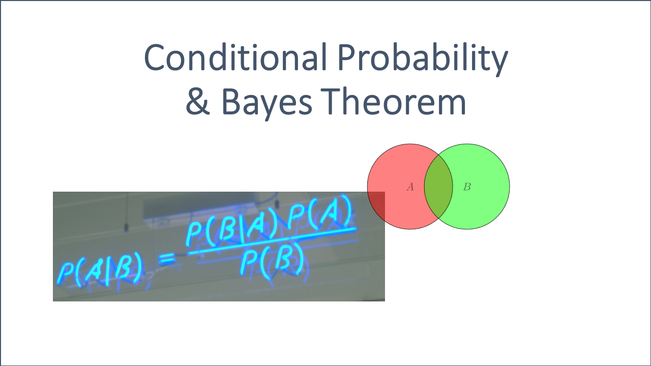
This article is about conditional probabilities and Bayes Rule / Theorem. In a second part, we are going to delve into conditional expectations.
Contents
Introduction
Conditional Probabilities and play a crucial role in various fields, including finance, economics, engineering, and data analysis. Conditional probabilities are a fundamental concept in probability theory that allows us to quantify the likelihood of an event occurring given certain conditions or information. They serve as a crucial tool for understanding and modeling events, providing valuable insights into complex systems across various domains, including statistics, machine learning, and decision analysis.
Conditional probability answers the question of ‘how does the probability of an event change if we have extra information’. It is therefore the foundation of Bayesian statistics.
Let us consider a probability measure ![]() of a measurable space
of a measurable space ![]() . Further, let
. Further, let ![]() , valid for the entire post.
, valid for the entire post.
Conditional Probability
Basics
Let us directly start with the formal definition of a conditional probability. Illustrations and explanations follow immediately afterwards.
Definition (Conditional Probability)
Let ![]() be a probability space and
be a probability space and ![]() . The real value
. The real value
(1) ![]()
is the probability of ![]() given that
given that ![]() has occurred or can be assumed.
has occurred or can be assumed. ![]() is the probability that both events
is the probability that both events ![]() and
and ![]() occur and
occur and ![]() is the new basic set since
is the new basic set since ![]() .
.
![]()
A conditional probability, denoted by ![]() , is a probability measure of an event
, is a probability measure of an event ![]() occurring, given that another event
occurring, given that another event ![]() has already occurred or can be assumed. That is,
has already occurred or can be assumed. That is, ![]() reflects the probability that both events
reflects the probability that both events ![]() and
and ![]() occur relative to the new basic set
occur relative to the new basic set ![]() as illustrated in Fig. 1.
as illustrated in Fig. 1.
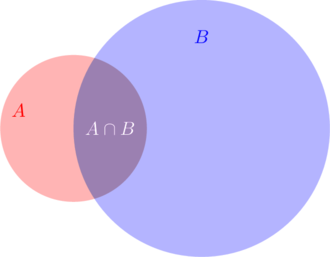
Figure 1: Venn diagram of a possible constellation of the sets ![]() and
and ![]()
The objective of ![]() is two-fold:
is two-fold:
- Determine the probability of
 while
while - Considering that
 has already occurred or can be assumed.
Latter item actually means ![]() since we know (by assumption, presumption, assertion or evidence) that
since we know (by assumption, presumption, assertion or evidence) that ![]() has been occurred or can be assumed. Graphically, the conditional probability
has been occurred or can be assumed. Graphically, the conditional probability ![]() is simply the relation between the intersection
is simply the relation between the intersection ![]() and the new basic set
and the new basic set ![]() .
.
Thereby we can clearly see that formula (1) is a generalization of the way how probabilities ![]() are calculated in general on
are calculated in general on ![]() .
.
![]() cannot be a null set since
cannot be a null set since ![]() . Due to the additivity of any probability space, we get
. Due to the additivity of any probability space, we get ![]() as
as ![]() . The knowledge about
. The knowledge about ![]() might be interpreted as an additional piece of information that we have received over time.
might be interpreted as an additional piece of information that we have received over time.
The following examples are going to illustrate this very basic concept.
Example 1.1 (Dice)
A fair dice is thrown once but it is not known what the outcome was. Let’s denote the event of rolling a ![]() or a
or a ![]() as
as ![]() . Furthermore, assume that it is known that the resulting number is an even number.
. Furthermore, assume that it is known that the resulting number is an even number.
How does the probability of getting ![]() change given the additional information?
change given the additional information?
Without the information ![]() , the proability of rolling an element of
, the proability of rolling an element of ![]() is
is ![]() since the dice is (assumed to be) fair. Using the additional information, however, changes the probability drastically as shown in the following.
since the dice is (assumed to be) fair. Using the additional information, however, changes the probability drastically as shown in the following.

The set of the event ![]() , where both conditions need to be fulfilled, is
, where both conditions need to be fulfilled, is
![]()
The corresponding probability on the basic set ![]() is
is ![]() . The probability of
. The probability of ![]() on
on ![]() equals
equals ![]() , such that we get
, such that we get ![]() .
.
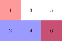
The corresponding situation is illustrated in the table above, where the set ![]() is highlighted in blue and
is highlighted in blue and ![]() in red. Hence, the intersection
in red. Hence, the intersection ![]() is highlighted in purple.
is highlighted in purple.
![]()
A heuristic that is sometimes applied to calculate ![]() is as follows:
is as follows:
Take the number of favorable outcomes and divide it by the total number of possible outcomes.
This heuristic is derived from the interpretation where ![]() is countable. If you consider the relative frequency (empirical probability)
is countable. If you consider the relative frequency (empirical probability) ![]() of the events
of the events ![]() and
and ![]() , then you derive the afore-mentioned heuristic. Note that
, then you derive the afore-mentioned heuristic. Note that ![]() denotes the power set of a given input set. We get
denotes the power set of a given input set. We get
![]()
Applied to Example 1.1, we can state that the total number of possible outcomes can be narrowed down to the set ![]() . Out of these only one is favorable and corresponds to rolling a 6. Notice that rolling a 1 is not favorable since it is not part of the set
. Out of these only one is favorable and corresponds to rolling a 6. Notice that rolling a 1 is not favorable since it is not part of the set ![]() . Hence, the result is
. Hence, the result is ![]() .
.
Probability Measure
Let us consider the probability measure derived from the conditional probability in more detail.
Theorem 1.1:
Let ![]() be a probability space,
be a probability space, ![]() and
and ![]() . The map
. The map
![]()
defines a probability measure on ![]() .
.
Proof:
Apparently, ![]() since
since ![]() and
and ![]() for all
for all ![]() . Further,
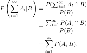
. Further, ![]() . The
. The ![]() -additivity follows by
-additivity follows by
![]()
Multiplication Rule
The following formula is called the multiplication rule and is simply a rewriting of formula (1) of the conditional probability.
(2) ![]()
Note that this formula also works if the events ![]() and
and ![]() are not independent, i.e. the multiplication rule is just a souped-up version of the rule of product, where two independent events are required.
are not independent, i.e. the multiplication rule is just a souped-up version of the rule of product, where two independent events are required.
The following example will illustrate this relationship.
Example 1.2 (Putting balls back to the urn)
An urn contains 5 white and 5 black balls. Two balls will be drawn successively without putting the balls back to the urn. We are interested in the event
![]() “red ball in the second draw”
“red ball in the second draw” ![]()
The probability of ![]() depends obviously on the result of the first draw. To find the probability of event
depends obviously on the result of the first draw. To find the probability of event ![]() (a red ball being drawn in the second draw), given that a red or a black ball was drawn in the first draw, we can use the concept of conditional probability. We distinguish the following two cases:
(a red ball being drawn in the second draw), given that a red or a black ball was drawn in the first draw, we can use the concept of conditional probability. We distinguish the following two cases:
- First draw results in a black ball, which is reflected in the event
 “First draw results in a black ball”
- First draw results in a red ball, which is reflected in the event
 “First draw results in a black ball”
Note that ![]() and that the events of drawing in the first and second round are dependent since the balls are not put back to the urn. Hence, we cannot use independence to calculate the denominator of formula (1). However, it is actually quite straight-forward to figure out the conditional probabilities
and that the events of drawing in the first and second round are dependent since the balls are not put back to the urn. Hence, we cannot use independence to calculate the denominator of formula (1). However, it is actually quite straight-forward to figure out the conditional probabilities ![]() as well as
as well as ![]() by simply using the relative frequencies heuristic.
by simply using the relative frequencies heuristic.
If the first draw resulted in a black ball, ![]() must be
must be ![]() since 4 black and 5 red balls are left. If the first draw resulted in a red ball instead,
since 4 black and 5 red balls are left. If the first draw resulted in a red ball instead, ![]() since 5 black and 4 red balls are left.
since 5 black and 4 red balls are left.
By knowing the conditional expectations, we can also conclude the probabilities of ![]() and
and ![]() via the multiplication rule even though the events are not mutually independent.
via the multiplication rule even though the events are not mutually independent.

![]()
Law of Total Probability
The Law of Total Probability relates the probability of an event ![]() to its conditional probabilities
to its conditional probabilities ![]() based on different “partitions” or “cases” of the sample space
based on different “partitions” or “cases” of the sample space ![]() . The “partitions” or “cases” are indexed by an index set
. The “partitions” or “cases” are indexed by an index set ![]() .
.
The theorem is often used to compute probabilities by considering categories that are mutually exclusive or disjoint.
Theorem 1.2 (Law of Total Probability):
Let ![]() be a probability space,
be a probability space, ![]() for all indizes
for all indizes ![]() with
with ![]() or
or ![]() and
and ![]() a partition of the basic set. Then
a partition of the basic set. Then

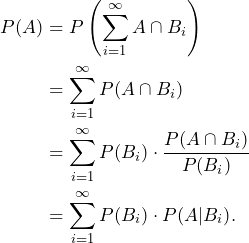
Proof: The equality of ![]() holds true for every set
holds true for every set ![]() . Due to the
. Due to the ![]() -additivity of
-additivity of ![]() , we can deduce
, we can deduce
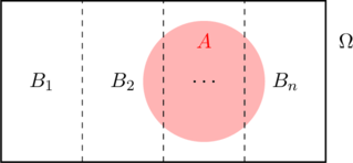
The situation with a finite index set ![]() is illustrated below.
is illustrated below.
![]()
The following lecture wraps it up and provides an example as well.
Let us consider also a quite simple and totally fictional example.
Example 1.3 (Math Enthusiast of a School Class)
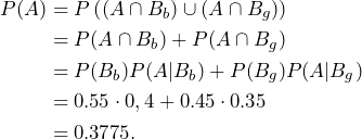
A class consists of 55% boys and 45% girls. 40% of the boys state that they are math enthusiast while 35% of the girls are excited by math. How likely is it to pick a math enthusiast of this particular school class?
Let us define the event ![]() {pick a math enthusiast of this school class}. Furthermore, we set
{pick a math enthusiast of this school class}. Furthermore, we set ![]() {set of kids that are boys} and
{set of kids that are boys} and ![]() {set of kids that are girls}. By applying the Law of Total Probability, we get
{set of kids that are girls}. By applying the Law of Total Probability, we get
![]()
Bayes Rule
The conditional probability ![]() is the probability that both events
is the probability that both events ![]() and
and ![]() occur relative to the new basic set
occur relative to the new basic set ![]() . Let us rearrange the conditional probability formula (1) as follows:
. Let us rearrange the conditional probability formula (1) as follows:

If we swap the roles of the sets ![]() and
and ![]() , formula (2) can furthermore be transformed into
, formula (2) can furthermore be transformed into

Let us pause here for a moment. Why does it make sense to actually swap the roles of the sets ![]() and
and ![]() ?
?
For two sets ![]() and
and ![]() , we can therefore conclude that
, we can therefore conclude that
(3) 
Now we are able to answer the question why it made sense to swap the roles of sets ![]() and
and ![]() . We were able to derive a formula that contains
. We were able to derive a formula that contains ![]() and
and ![]() . Hence, we have derived a formula which conects the probability of the original
. Hence, we have derived a formula which conects the probability of the original ![]() with the situation after we have received additional information
with the situation after we have received additional information ![]() and that the probability
and that the probability ![]() encodes this.
encodes this.
Formula (3) is a special case of Bayes’ Rule or Bayes’ Theorem. Let us formulate the more general theorem.
Theorem 1.3 (Bayes’ Theorem):
Let ![]() be a probability space,
be a probability space, ![]() for all indizes
for all indizes ![]() with
with ![]() or
or ![]() and
and ![]() a partition of the basic set. Then
a partition of the basic set. Then

Proof: Use the before mentioned argumentation for the more general case.
![]()
Example 2.1 (Medical Test for Rare Desease)
Suppose there is a rare disease that affects only 1 in 1000 people, i.e. there is a probability of 0,01% to catch the disease. A medical test has been developed to diagnose this disease. The test is highly accurate as it correctly identifies the disease 99% of the time (sensitivity), and it correctly also identifies the absence of the disease (specification) 99% of the time.
Let us define the folllowing events/sets:
- Event
 : a person has the disease
 - Event
 : a person does not have the disease.
This event is the complementary event of
- Event
 : the medical test is positive
We want to find the probability that a person who tests positive actually has the disease, ![]() .
.
Bayes’ Theorem helps us figure out the probability that someone actaully has a disease ![]() given that they have tested positive
given that they have tested positive ![]() . This is important because even though a test might be accurate, it is possible for false positives to happen. That is,
. This is important because even though a test might be accurate, it is possible for false positives to happen. That is,
![]()
where
 is the probability of testing positive given that a person has the disease. This is the sensitivity of the test, which is 0.99 in this case.
  is the prior probability of having the disease, which is 0.001 (1 in 1000 people)
 is the probability of testing positive. Given that a test can be positive, when a person doesn’t have the disease. We therefore need to consider both scenarios and apply the Law of Total Probability when calculating

Note that ![]() is the probability of testing positive given that a person doesn’t have the disease. This is 1 minus the specificity, so
is the probability of testing positive given that a person doesn’t have the disease. This is 1 minus the specificity, so ![]() = 1 – 0.99 = 0.01. In addition,
= 1 – 0.99 = 0.01. In addition, ![]() is the probability of not having the disease, which is
is the probability of not having the disease, which is ![]() .
.
Putting it all together we get
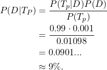
Image you have a sample of 1000 people as illustrated by the dots in Fig. 1. One out of 1000 actually has the disease and is correctly identified by the test. Another 10 are falsely identified and actually do not have the disease. In total 11 people have been tested positive, but only one actually has the disease, i.e., ![]() .
.

Figure 1: Sample of 1000 people where one is true positive and 10 are false positive.
![]()
Formula (3) is also called Bayes’ Rule or Bayes’ Theorem.


