
Contents
Introduction
Copulas are an important concept in statistics and beyond to describe dependency structures of continuous distributions. However, what can we do if we have multivariate data at hand. And how can we do that?
The following blog post provides a hands-on approach to empirical copulas. It provides insight and illustrations.
Let us assume we have a sample of two random variables  and
and  at hand, and we would like to know more about how both variables are interrelated to each other. The elements of the sample of size
  of both random variables shall be denoted as a tuple
  with
with  .
.
The empirical (bivariate) copula is defined as the discrete function  given by
(1) 
where  and
and  ,
,  denote the order statistics of the sample and
  provides the cardinality of the subsequent set. For instance,
  .
.
Notice that the definition is actually a special case of the definition of an empirical distribution function. However, empirical copula functions are only defined on ![[0,1]^n](https://www.deep-mind.org/wp-content/ql-cache/quicklatex.com-8c7e5ef3eee1d86a6f847384cc30f7f3_l3.png "Rendered by QuickLaTeX.com") and they represent a dependency structure and not a distribution.
and they represent a dependency structure and not a distribution.
Hands-on Approach
Uniformly with a sample size of n=5
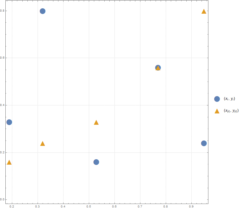
First, let us assume that and follow an uniform distribution on ![[0,1]](https://www.deep-mind.org/wp-content/ql-cache/quicklatex.com-0621f04d8a0d9e76a5abce6204d5b435_l3.png "Rendered by QuickLaTeX.com") . For both random variables we draw a small sample of size
. For both random variables we draw a small sample of size  . The sample is listed in the following table and illustrated in the plot below (blue points).
 |
 |
 |
|
|
|---|---|---|---|---|
| 1 | 0.95 | 0.24 | 0.19 | 0.16 |
| 2 | 0.53 | 0.16 | 0.32 | 0.24 |
| 3 | 0.77 | 0.56 | 0.53 | 0.33 |
| 4 | 0.19 | 0.33 | 0.77 | 0.56 |
| 5 | 0.32 | 0.80 | 0.95 | 0.80 |
According to the definition of the empirical copula, we also need to know the corresponding ordered samples and , which can also be found in the table above. In addition, the tuples of the order statistic  are also sketched in the plot below (orange triangles).
 as well as of the order statistic
The domain of the empirical copula is the Cartesian product of the values  . For instance,
  since no tupel exists such that
  and
and  for
for  . However, for
  and
and  the tuple
  meet the conditions
  and
and  with
with  .
.
By knowing the set in the numerator of equation (1), we are able to derive the corresponding empirical copula value easily. We just need to count the elements of this set and divide the number by the sample size . The result is the desired empirical copula value which is a (cumulative) frequency.
Note that the set of equation (1) corresponds to all points  that lie within the rectangles intersecting the
  and
and  axes, respectively, passing through
  .
.
The values  are listed in the following table.
|
 |
 |
 |
 |
 |
|---|---|---|---|---|---|
|
0.00 | 0.00 | 0.20 | 0.20 | 0.20 |
|
0.00 | 0.00 | 0.20 | 0.20 | 0.40 |
|
0.20 | 0.20 | 0.40 | 0.40 | 0.60 |
|
0.20 | 0.20 | 0.40 | 0.60 | 0.80 |
|
0.20 | 0.40 | 0.60 | 0.80 | 1.00 |
Graphically the empirical copula looks as follows:
 where both variables are distributed uniformly on
 Normally distributed with a sample size of n=100
Second, let us now assume that  follows a bivariate normal distributed with mean
  and
and
![\[ \Sigma := \left(\begin{array}{ccc} 1 & \rho \\ \rho & 1 \\ \end{array}\right) \]](https://www.deep-mind.org/wp-content/ql-cache/quicklatex.com-35532bf30a7487578326878862385e21_l3.png "Rendered by QuickLaTeX.com")
.
Here,  is the correlation coefficient between and . We draw a bivariate sample of size
  with
with  using R.
library(mvtnorm) #package to simulate joint normal distribution
n <- 100 #sample size
# parameters of the bivariate normal
mean <- c(0,0) # mean for distribution
sigma <- matrix(c(1,0.3,0.3,1), ncol=2) # correlation matrix
# sample the bivariate normal
Z <- rmvnorm(n=n, mean = mean, sigma = sigma) # simulate bivariate normally distributed sample
plot(Z, main="Bivariate Normal, Correlation 0.3, X vs. Y")
# divide Z to get X and Y
X <- Z[,1]
Y <- Z[,2]
# sort sample
X.ascending <- sort(X)
Y.ascending <- sort(Y)
Z.ascending <- cbind(X.ascending, Y.ascending)
# prepare data structure
C.n <- as.data.frame(matrix(nrow = n, ncol = n), row.names = paste0("X", 1:n))
colnames(C.n) <- paste0("Y", 1:n)
# run through the indizes i (of X) and j (of Y)
for( i in 1:n){
for( j in 1:n){
C.n[i, j] <- sum(apply(X=Z, MARGIN = 1, FUN = function(Z.row, x.sorted, y.sorted) { sum(Z.row <= c(x.sorted, y.sorted), na.rm = TRUE) >=2 }, X.ascending[i], Y.ascending[j]), na.rm = TRUE)/n
}
}
# plot the empirical copula
library(plot3D)
x <- (1:n)/n
y <- x
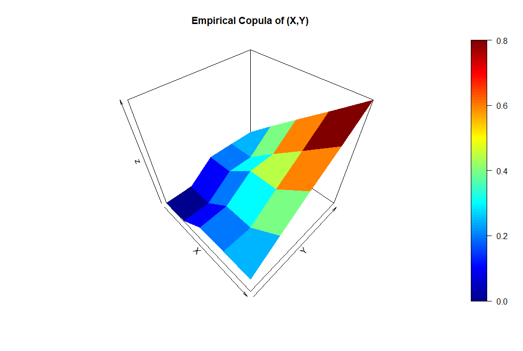
persp3D(x = x, y = y, z = as.matrix(C.n), phi = 45, theta = 45, xlab = "X", ylab = "Y", main = "Empirical Copula")
We basically apply the same algorithm to calculate the empirical copula values, which are computed within the loops and named by C.n[i, j]. The arguments i and j represent the values of the domain of the empirical copula. The defined function then just counts whether what conditions are met and divides by .
The plot created by R (for my specific random variate) can be seen in the following.
Transforming the normally distributed sample
Let us further use the random sample with  that we have just simulated. However, let us define new random variables
  and
and  by transforming the samples
  ,
,  with
with  accordingly.
What do you think how the corresponding empirical copula will look like?
Well, given that  is a monotone function nothing will change since the order of the sample will not change. The following R code demonstrates that.
library(mvtnorm) #package to simulate joint normal distribution
library(mvtnorm) #package to simulate joint normal distribution
n <- 100 #sample size
# parameters of the bivariate normal
mean <- c(0,0) # mean for distribution
sigma <- matrix(c(1,0.3,0.3,1), ncol=2) # correlation matrix
# sample the bivariate normal
Z <- rmvnorm(n=n, mean = mean, sigma = sigma) # simulate bivariate normally distributed sample
plot(Z, main="Bivariate Normal, Correlation 0.3, X vs. Y")
# divide Z to get X and Y
X <- Z[,1]
Y <- Z[,2]
cor(X,Y)
# apply a monotone transformation to X and Y
R <- exp(X)
S <- exp(Y)
cor(R, S)
T <- cbind(R, S)
# sort simulated sample
X.ascending <- sort(X)
Y.ascending <- sort(Y)
Z.ascending <- cbind(X.ascending, Y.ascending)
# sort transformed sample
R.ascending <- sort(R)
S.ascending <- sort(S)
T.ascending <- cbind(R.ascending, S.ascending)
# prepare data structures
C.n <- as.data.frame(matrix(nrow = n, ncol = n), row.names = paste0("X", 1:n))
colnames(C.n) <- paste0("Y", 1:n)
C.n.trans <- as.data.frame(matrix(nrow = n, ncol = n), row.names = paste0("R", 1:n))
colnames(C.n.trans) <- paste0("S", 1:n)
# run through the indizes i (of X/R) and j (of Y/S)
for( i in 1:n){
for( j in 1:n){
C.n[i, j] <- sum(apply(X=Z, MARGIN = 1, FUN = function(Z.row, x.sorted, y.sorted) { sum(Z.row <= c(x.sorted, y.sorted), na.rm = TRUE) >=2 }, X.ascending[i], Y.ascending[j]), na.rm = TRUE)/n
C.n.trans[i, j] <- sum(apply(X=T, MARGIN = 1, FUN = function(T.row, r.sorted, s.sorted) { sum(T.row <= c(r.sorted, s.sorted), na.rm = TRUE) >=2 }, R.ascending[i], S.ascending[j]), na.rm = TRUE)/n
}
}
# plot the empirical copula
library(plot3D)
x <- (1:n)/n
y <- x
par(mfrow=c(1, 2)); #prepare canvas
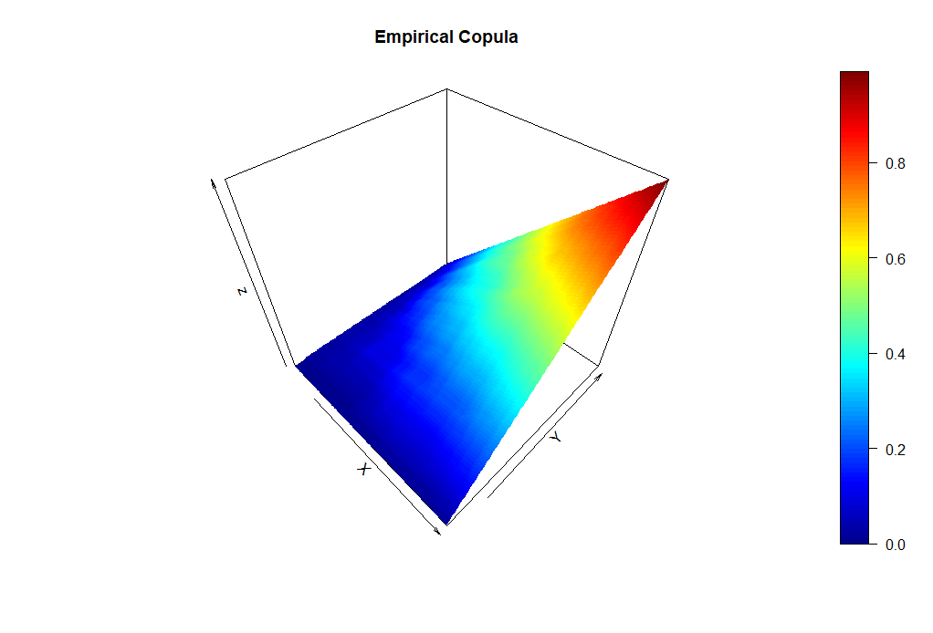
persp3D(x = x, y = y, z = as.matrix(C.n), phi = 45, theta = 45, xlab = "X", ylab = "Y", main = "Empirical Copula of (X,Y)")
persp3D(x = x, y = y, z = as.matrix(C.n.trans), phi = 45, theta = 45, xlab = "Exp(X)", ylab = "Exp(Y)", main = "Empirical Copula of (Exp(X), Exp(Y))")
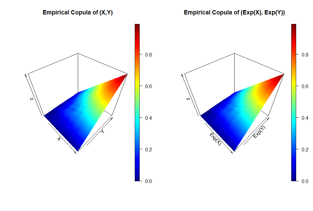 and transformed
The comparison of both plots show graphically that the empirical copula does not change by the transformation.
For all who would like to know more about empirical copulas I recommend [1] by Genest et al.