Introduction
The quantification and even the definition of ‘risk’ is a hard problem. Questions like the following are therefore–in general–hard to answer:
- What is the risk of investing in a the Euro Stoxx 50?
- What is the risk that there will be a war between Taiwan and China?
- What is the default risk of Apple Inc.?
- …
In this post, we recap the general properties of a risk measure as derived in the seminal paper “Coherent Measures of Risk” [1] by Philippe Artzner, Freddy Delbaen, Jean-Marc Eber and David Heath. We will focus on outlining the heuristic behind the concept of coherent risk measures by connecting it to practice and providing illustrative examples. To this end, we follow mainly the structure of the outstanding book [2] by Föllmer & Schied. In addition, we will also extend the basic idea of coherent to convex risk measures as suggested by Föllmer & Schied [2].
The focus is on the general properties of measures of risk and its applications and connections to other areas of math (finance). Concrete risk measures such as Worst-Case Risk Measure, Value at Risk or Expected Shortfall will serve as examples but are not in the main focus of this post.
Note that, if we define a concrete risk measure such as the Value at Risk, then the term “risk” is implicitly defined by the conducted calculation.
Monetary Risk Measures
The main objective of a risk measure ![]() is to quantify the risk of any financial position
is to quantify the risk of any financial position ![]() . By applying a risk measure, we are then able to ‘compare’ the riskiness of different financial positions. The precise meaning of a financial position is left unspecified but may include assets, liabilities, and any kind other financial instrument such as derivatives.
. By applying a risk measure, we are then able to ‘compare’ the riskiness of different financial positions. The precise meaning of a financial position is left unspecified but may include assets, liabilities, and any kind other financial instrument such as derivatives.
Let ![]() be a fixed set of scenarios, that are needed for the valuation of a financial position
be a fixed set of scenarios, that are needed for the valuation of a financial position ![]() . The set
. The set ![]() is also called the set of states of nature or states of the world. Refer also to the post about the notation of decision problems.
is also called the set of states of nature or states of the world. Refer also to the post about the notation of decision problems.
One scenario ![]() might be represented by cash flows of the financial position rolled out on a timeline that stretches from inception
might be represented by cash flows of the financial position rolled out on a timeline that stretches from inception ![]() until the end
until the end ![]() of the risk horizon. These cash flows dependent on a specific scenario
of the risk horizon. These cash flows dependent on a specific scenario ![]() can also be interrelated to indicators such as an interest environment, specific macro-economic developments or the foreign exchange rates.
can also be interrelated to indicators such as an interest environment, specific macro-economic developments or the foreign exchange rates.
A financial position is defined by a mapping ![]() , where
, where ![]() is the discounted net worth of the position at the end of the risk horizon if the scenario
is the discounted net worth of the position at the end of the risk horizon if the scenario ![]() is realized. Positive values of
is realized. Positive values of ![]() denote profits while negative values denote losses accrued over
denote profits while negative values denote losses accrued over ![]() .
.

That is, ![]() is the net cash flow of the financial position based on all possible scenarios
is the net cash flow of the financial position based on all possible scenarios ![]() with their net worth
with their net worth ![]() . The associated risk
. The associated risk ![]() of a financial position
of a financial position ![]() under a given scenario
under a given scenario ![]() is also dependent on the reporting date.
is also dependent on the reporting date.
Example 2.1 (Present Value of a Coupon Bond)
Let us assume we have invested mn€ 100 in one bond with a 2% coupon and a maturity of 5 years. That is, the financial position ![]() comprises only the single bond and we receive the annual interest payment of mn€ 2 for five consecutive years. If the counterparty will not default, we also receive the notional at maturity.
comprises only the single bond and we receive the annual interest payment of mn€ 2 for five consecutive years. If the counterparty will not default, we also receive the notional at maturity.
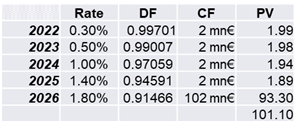
The scenario ![]() is represented by the development of the issuer-specific interest rate levels as reflected in column “Rate” of Tab. 1. Note that these specific interest rate for that particular bond comprises all types of risk including the general interest rate risk, the credit spread risk as well as the liquidity situation of the corresponding market.
is represented by the development of the issuer-specific interest rate levels as reflected in column “Rate” of Tab. 1. Note that these specific interest rate for that particular bond comprises all types of risk including the general interest rate risk, the credit spread risk as well as the liquidity situation of the corresponding market.
Due to the fact that the reference interest rates for all terms are below the issuer-specific 2% coupon, the bond is valued above 100.
The present value of ![]() is also implicitly given in Tab. 1 by its bond price denoted in %. Since we are ultimately interested in the net present value (i.e. the P&L) we need to deduct the initial price of
is also implicitly given in Tab. 1 by its bond price denoted in %. Since we are ultimately interested in the net present value (i.e. the P&L) we need to deduct the initial price of ![]() that we paid for the bond portfolio. Hence,
that we paid for the bond portfolio. Hence, ![]()
A functional ![]() connects the scenarios of the basic set
connects the scenarios of the basic set ![]() with its related net present value. Thereby, it doesn’t really matter how
with its related net present value. Thereby, it doesn’t really matter how ![]() exactly looks like. It can comprise the risk factors that are needed for the valuation or some macroeconomic scenarios where we know how these fluctuations will impact the net worth of the position.
exactly looks like. It can comprise the risk factors that are needed for the valuation or some macroeconomic scenarios where we know how these fluctuations will impact the net worth of the position.
![]()
Recall that a functional is a mapping from a (vector) space into a field of scalars. Hereby, the field of scalars is the real line with the usual addition and multiplication, denoted by ![]() .
.
The collection of all financial positions, denoted by ![]() , therefore comprises a function vector space equipped with the usual operations of a function space. The main task of this function space is to provide the environment for the valuation of all financial positions as of a given reporting date.
, therefore comprises a function vector space equipped with the usual operations of a function space. The main task of this function space is to provide the environment for the valuation of all financial positions as of a given reporting date.
If ![]() , the set of all financial positions
, the set of all financial positions ![]() can also be identified with
can also be identified with ![]() . In this case, all financial positions can only have
. In this case, all financial positions can only have ![]() function values, which means that we can define a bilateral mapping between the function values and
function values, which means that we can define a bilateral mapping between the function values and ![]() .
.
A financial position ![]() also needs to be bounded and all constant functions need to be contained in
also needs to be bounded and all constant functions need to be contained in ![]() . Latter requirement reflects the existence of financial positions, that are (assumed to be) not subject to fluctuations and can therefore be considered as risk-free. The boundedness of any financial position is also reasonable since we live in a finite world and thus every valuation of a real-world asset also needs to be finite. Refer to the famous St. Petersberg paradox in this context.
. Latter requirement reflects the existence of financial positions, that are (assumed to be) not subject to fluctuations and can therefore be considered as risk-free. The boundedness of any financial position is also reasonable since we live in a finite world and thus every valuation of a real-world asset also needs to be finite. Refer to the famous St. Petersberg paradox in this context.
Our objective is to quantify the risk of any financial position ![]() by a risk measure
by a risk measure ![]() defined by
defined by ![]() . This means, that we need to ‘compare’ the valuations of the financial positions with each other using the order relation and think about their implications on risk.
. This means, that we need to ‘compare’ the valuations of the financial positions with each other using the order relation and think about their implications on risk.
Definition 2.1 (Dominance & Order of Functions)
Let ![]() be a function space and
be a function space and ![]() . We say that
. We say that ![]() is dominated by
is dominated by ![]() , or
, or ![]() dominates
dominates ![]() , if
, if ![]() for all scenarios
for all scenarios ![]() .
.
![]()
The finitary relation ‘![]() ‘ as outlined in Definition 2.1 on the function space
‘ as outlined in Definition 2.1 on the function space ![]() is a partial and even a total order. Note that the comparison actually takes place in
is a partial and even a total order. Note that the comparison actually takes place in ![]() employing the canonical or usual order on the real line.
employing the canonical or usual order on the real line.
Definition 2.2 (Monetary Measure)
A mapping ![]() is called a monetary measure of risk if it satisfies the following conditions for all
is called a monetary measure of risk if it satisfies the following conditions for all ![]() .
.
(i) Monotonicity: If ![]() , then
, then ![]() ;
;
(ii) Cash or Translation Invariance: If ![]() , then
, then ![]() .
.
![]()
Note that no probability measure has been used in this definition. We are simply working on a function space with certain properties. That is, ![]() means that we add an arbitrary function and a constant function together using the vector addition as defined on the function space.
means that we add an arbitrary function and a constant function together using the vector addition as defined on the function space.
By definition, risk is denoted as a positive while chance is denoted as negative figure.
The economic meaning of both properties (i) and (ii) are as follows:
(i) Monotonicity:
The risk ![]() of the position
of the position ![]() is reduced when the payoff profile
is reduced when the payoff profile ![]() is increased compared to
is increased compared to ![]() ;
;
(ii) Cash or Translation Invariance:
Cash is considered to be risk free since it is deposited at central banks at the end of each business day by banks. In addition, ![]() can be interpreted as some sort of capital requirement (imposed by a regulator). Common Equity Tier 1 Capital needs to be in some cash-like form.
can be interpreted as some sort of capital requirement (imposed by a regulator). Common Equity Tier 1 Capital needs to be in some cash-like form.
Cash invariance implies
![]()
since ![]() as part of the argument of the function can be considered as a constant. That is, sufficient cash/capital is added to neutralize the risk
as part of the argument of the function can be considered as a constant. That is, sufficient cash/capital is added to neutralize the risk ![]() completely. We can also conclude that
completely. We can also conclude that
![]()
for all ![]() . That is, a cash amount
. That is, a cash amount ![]() is reducing the risk by the same amount as we have seen in just above.
is reducing the risk by the same amount as we have seen in just above.
We also say that the risk has become acceptable (by supervisory authorities, for example). It also implies ![]() for all
for all ![]() .
.
For most purposes it wouldn’t be a loss of generality to assume that a given monetary risk measure satisfies the condition of
Normalization: ![]() .
.
Since the argument of the monetary measure ![]() represents the discounted net worth, the zero vector
represents the discounted net worth, the zero vector ![]() tells us that this kind of investment would not imply any benefit no matter what scenario would realize.
tells us that this kind of investment would not imply any benefit no matter what scenario would realize.
Convex & Coherent Risk Measures
Why should a risk measure be convex and what does it actually mean?
The convexity property of a monetary measure of risk restricts the risk values of sub-portfolios with respect to the corresponding overarching portfolio. Before we come to convex risk measures, let us recall what convex sets and functions are.
Definition 3.1 (Convex Set & Convex Function)
A set ![]() is convex if for all
is convex if for all ![]() , and
, and ![]() , we have
, we have
![]()
A point of that form ![]() ,
, ![]() is called convex combination of
is called convex combination of ![]() and
and ![]() .
.
A function ![]() is convex if its domain is a convex set and for all
is convex if its domain is a convex set and for all ![]() , and
, and ![]() , we have
, we have
![]()
![]()
If we take any two points ![]() , then
, then ![]() evaluated at any convex combination of these two points should be no larger than the same convex combination of
evaluated at any convex combination of these two points should be no larger than the same convex combination of ![]() and
and ![]() . Geometrically, the line segment connecting
. Geometrically, the line segment connecting ![]() to
to ![]() must sit above the graph of
must sit above the graph of ![]() . A convex combination of the two points
. A convex combination of the two points ![]() to
to ![]() can be considered as a line segment (i.e. a chord) between the points. Thereby, the convex combination with
can be considered as a line segment (i.e. a chord) between the points. Thereby, the convex combination with ![]() form the end-points
form the end-points ![]() to
to ![]() of the line segment. The remaining convex combinations generate the points in between these two end points.
of the line segment. The remaining convex combinations generate the points in between these two end points.
Example 3.1 (Quadratic Function)
The function ![]() defined on the domain
defined on the domain ![]() is convex, which can directly be seen geometrically.
is convex, which can directly be seen geometrically.

In the sketched graph of ![]() , we can see several example chords that connect two points on the graph. All of these chords sit above the the graph of
, we can see several example chords that connect two points on the graph. All of these chords sit above the the graph of ![]() as required by the interpretation of the convexity property.
as required by the interpretation of the convexity property.
In order to illustrate the convexity property, let us fix two points on the graph that imply the chord between them. Convexity now tells us that ![]() (green point) is equal or smaller than
(green point) is equal or smaller than ![]() (blue point) at
(blue point) at ![]() .
.

The convex combination of the function values therefore sits above the graph on the chord while the convex combination of the arguments will be mapped on the graph of ![]() .
.
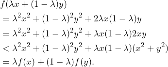
Let us now proof algebraically that the function ![]() is convex.
is convex.
The function ![]() is convex on
is convex on ![]() . Let us apply the definition of the function and convexity to see this:
. Let us apply the definition of the function and convexity to see this:

Due to the fact that ![]() we imply that
we imply that ![]() and thus
and thus ![]() . By adding
. By adding ![]() , we get the inequality
, we get the inequality ![]() which can be applied to
which can be applied to
![]()
Let us now apply convex functions to monetary risk measures.
Definition 3.1 (Convex Risk Measure)
A monetary risk measure ![]() is called a convex measure of risk if for all real
is called a convex measure of risk if for all real ![]() the following holds true.
the following holds true.
(iii) Convexity: ![]() .
.
![]()
The entire financial position is represented by ![]() . However, let us consider the isolated sub-portfolios of the financial positions
. However, let us consider the isolated sub-portfolios of the financial positions ![]() and
and ![]() , where
, where ![]() and
and ![]() has been invested into
has been invested into ![]() and
and ![]() , respectively.
, respectively.
The convexity property (iii) states that the risk ![]() of a portfolio is not greater than the weighted sum of the risk of its constitutes. That is, diversification in a given portfolio
of a portfolio is not greater than the weighted sum of the risk of its constitutes. That is, diversification in a given portfolio ![]() does not increase the risk
does not increase the risk ![]() and is therefore not greater than
and is therefore not greater than ![]() .
.
In general, this assumptions does make sense since diversification should decrease risk. Just think about the idiom “Do not put all our eggs in one basket“.
Before we dive further into convex risk measures, let us recall the concept of linear cones. We will see that there is a one-to-one connection between convex risk measures and linear cones.
Definition 3.2 (Linear or Convex Cone)
Let ![]() be a real vector space. A non-empty subset
be a real vector space. A non-empty subset ![]() is called a cone if it is closed under multiplication by non-negative scalar, i.e. if
is called a cone if it is closed under multiplication by non-negative scalar, i.e. if ![]() for each scalar
for each scalar ![]() .
.
![]()
Let us have a look at simple examples.
Example 3.3 (Cones)
(a) The non-negative number tuples in the quarter plane ![]() forms a cone. Every point
forms a cone. Every point ![]() can be scaled with
can be scaled with ![]() arbitrarily, such that the entire quarter is comprised by the cone
arbitrarily, such that the entire quarter is comprised by the cone ![]() .
.
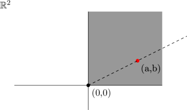
For the sake of simplicity, the highlighted area is finite but the actual area of ![]() , of course, is infinite.
, of course, is infinite.
(b) Any wedge which extends to infinity from the origin is a cone in ![]() .
.
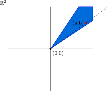
Note that the sketch is simplified since the highlighted area is finite even though the wedge ![]() is not bounded as indicated by the dashed line.
is not bounded as indicated by the dashed line.
(c) Given any finite number of vectors ![]() in a real vector space, the conical combination
in a real vector space, the conical combination

forms a convex set and a cone.
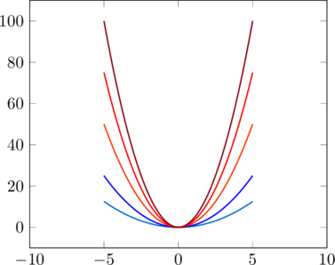
(d) In any function space, the set ![]() is a cone since the function
is a cone since the function ![]() for all
for all ![]() . So,
. So, ![]() . Let us consider the scaling effect with scalars
. Let us consider the scaling effect with scalars ![]() on the positive function
on the positive function ![]() that is sketched in dark blue.
that is sketched in dark blue.
![]()
For more details and further definitions and theorems about linear cones please refer to [5].
The analog property to be closed under multiplication by non-negative scalar is called positive homogeneity for functions.
Definition 3.3 (Coherent Risk Measure)
A convex risk measure ![]() is called a coherent measure of risk if it satisfies
is called a coherent measure of risk if it satisfies
(iv) Positive Homogeneity:![]() for all
for all ![]() .
.
![]()
If a monetary measure of risk ![]() is positively homogeneous, then it is normalized with
is positively homogeneous, then it is normalized with ![]()
![]()
In addition, property (iv) tells us that the risk grows by the same proportion ![]() if we scale our portfolio by
if we scale our portfolio by ![]() . Loosely speaking, by doubling a portfolio the corresponding risk will also be doubled.
. Loosely speaking, by doubling a portfolio the corresponding risk will also be doubled.
The assumption (iv) might be questionable since risk might not increase linearly when we scale up the portfolio by the same factor. A possible cause for an increasing risk can be a decreasing degree of liquidity. Please note that Artzner et al [1] was aware of that model limitation of coherent risk measures:
Of course, this assumes that markets at date
are liquid; if they are not, more complicated models are required, where we can distinguish the risk of a position from and of a future net worth, since, with illiquid markets, the mapping from the former to the latter may not be linear.
— Section 2.2 in [1]
Under the assumption of positive homogeneity, convexity is equivalent to
(v) Subadditivity: ![]() .
.
To see this, let us consider a convex risk measure ![]() that is also positive homogeneous. By setting
that is also positive homogeneous. By setting ![]() , we can derive
, we can derive

which shows the sub-linearity simply by applying the convexity and the homogeneity property. The choice of ![]() is required to have a portfolio with an equal share of financial positions
is required to have a portfolio with an equal share of financial positions ![]() and
and ![]() . It is then possible to scale up these proportions to the required size of 1 unit for both financial positions.
. It is then possible to scale up these proportions to the required size of 1 unit for both financial positions.
![]()
Subadditivity reflects the idea that risk cannot be increased by diversification and that risk can be scaled up proportionally with the size of a portfolio. If separate risk limits are assigned to separate ‘(trading) desks’, then the risk of the aggregate position is bounded by the sum of the individual risk limits.
Acceptance Sets & Risk Measures
Let us now put ourselves into the shoes of a supervisory authority. Regulators such as EBA, ECB, PRA, etc. want to is to prevent or mitigate systemic risks to the financial system as a whole.
Regulated financial institutions usually need to determine and reserve capital requirements in a particular process to ensure the soundness of the regulated financial system. In Europe, this process is called Internal Capital Adequacy Assessment Process, short ICAAP. The main purpose of this process is to calculate the capital requirement of the aggregated risk positions for a financial institution. If this capital is reserved for that particular purpose, the financial position is considered to be acceptable from a regulator’s and/or an investor’s point of view.
Definition 4.1 (Acceptance Set)
A financial position ![]() with respect to a monetary measure
with respect to a monetary measure ![]() is said to be acceptable if
is said to be acceptable if ![]() and not acceptable otherwise. A monetary measure
and not acceptable otherwise. A monetary measure ![]() induces the class
induces the class
![]()
of positions, which are acceptable in the sense that it does not require any additional capital. The class ![]() will be called the acceptance set of
will be called the acceptance set of ![]() .
.

![]()
That is, an acceptable financial position needs to comprise the capital requirements in some form of cash. Let us consider this simple example further.
Example 4.1 (Acceptable and Unacceptable Position)
Assume that a financial institution holds a risky position ![]() and
and ![]() is a corresponding coherent risk measure. The position
is a corresponding coherent risk measure. The position ![]() entails a not acceptable risk of
entails a not acceptable risk of ![]() . That is, if we add cash as a capital reserve to the financial position of
. That is, if we add cash as a capital reserve to the financial position of ![]() , then we receive an acceptable position
, then we receive an acceptable position ![]() since
since ![]() .
.
![]()
The following two propositions summarize the relationship between monetary measures of risk and their acceptance sets.
Proposition 4.1 (Monetary Measure & Acceptance Sets)
Suppose that ![]() is a monetary measure of risk with acceptance set
is a monetary measure of risk with acceptance set ![]() .
.
(a) ![]() is non-empty, and satisfies the following two conditions:
is non-empty, and satisfies the following two conditions:
(1) ![]()
(2) ![]()
If ![]() the following set
the following set
(3) ![]()
(b) The monetary measure of risk ![]() can be recovered from
can be recovered from ![]() via
via
(4) ![]()
Proof. (a) We show that ![]() takes only finite values. To this end, fix some
takes only finite values. To this end, fix some ![]() in the non-empty set
in the non-empty set ![]() . For a
. For a ![]() given, there exists a finite number
given, there exists a finite number ![]() with
with ![]() , because
, because ![]() and
and ![]() are both bounded. Then
are both bounded. Then
![]()
and hence ![]() . Note that (1) is equivalent to
. Note that (1) is equivalent to ![]() . To show that
. To show that ![]() for arbitrary
for arbitrary ![]() , we take
, we take ![]() such that
such that ![]() and conclude by monotonicity and cash invariance that
and conclude by monotonicity and cash invariance that ![]() .
.
As an accepted position ![]() , it’s risk value needs to fulfill the condition
, it’s risk value needs to fulfill the condition ![]() . If
. If ![]() and
and ![]() then
then ![]() due to monotonicity. Hence,
due to monotonicity. Hence, ![]() also needs to be acceptable.
also needs to be acceptable.
The function ![]() for
for ![]() is continuous such that
is continuous such that
![]()
is closed. Refer to Theorem 5.1 and 5.5 for further details.
(b) Applying the cash translation invariance, we can derive the following chain of equations.
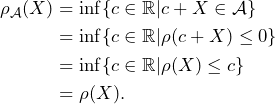
If ![]() then
then ![]() has to be equal to
has to be equal to ![]() since any smaller value would not imply an acceptable set and and bigger value would not be the infimum.
since any smaller value would not imply an acceptable set and and bigger value would not be the infimum.
![]()
Implication (2) in the Proposition 4.1 means the following: if a financial position ![]() is acceptable and we consider another financial position
is acceptable and we consider another financial position ![]() , where the net cash flow profile is greater or equal to
, where the net cash flow profile is greater or equal to ![]() , then
, then ![]() also needs to be acceptable. Consider that
also needs to be acceptable. Consider that ![]() means that an investor gets its money back more quickly such that the risk can only be lower.
means that an investor gets its money back more quickly such that the risk can only be lower.
As mentioned in (b) of the last proposition, we can take a given class ![]() of acceptable positions and define the risk as the minimal amount
of acceptable positions and define the risk as the minimal amount ![]() for which the position
for which the position ![]() becomes acceptable.
becomes acceptable.
Definition 4.2 (Capital Requirement)
The minimal amount ![]() –as defined in (4)– for which the position
–as defined in (4)– for which the position ![]() becomes acceptable is called capital requirement and the map
becomes acceptable is called capital requirement and the map ![]() with
with ![]() is called capital requirement measure.
is called capital requirement measure.
![]()
The following proposition will show that the capital requirement measure is a monetary measure of risk.
Proposition 4.2 (Convex Risk Measure)
Suppose that ![]() is a non-empty subset of
is a non-empty subset of ![]() which satisfies (1) and (2). Then the functional
which satisfies (1) and (2). Then the functional ![]() has the following properties:
has the following properties:
(a) ![]() is a monetary measure of risk.
is a monetary measure of risk.
(b) If ![]() is a convex set, then
is a convex set, then ![]() is a convex measure of risk.
is a convex measure of risk.
(c) If ![]() is a cone, then
is a cone, then ![]() is positively homogenous. In particular,
is positively homogenous. In particular, ![]() is a coherent measure of risk if
is a coherent measure of risk if ![]() is a convex cone.
is a convex cone.
(d) The monetary measure of risk ![]() is convex if and only if
is convex if and only if ![]() is convex.
is convex.
(e) The monetary measure of risk ![]() is positively homogeneous if and only if
is positively homogeneous if and only if ![]() is a cone. In particular,
is a cone. In particular, ![]() is coherent if and only if
is coherent if and only if ![]() is a convex cone.
is a convex cone.
Proof. (a) First of all, consider that (1) as well as (2) are assumed to be valid. According to (b) of Proposition 4.1, the following equation is valid.
![]()
Since ![]() is cash translation invariant so is
is cash translation invariant so is ![]() . The monotonicity follows from the same argument and (2).
. The monotonicity follows from the same argument and (2).
(b) Suppose that ![]() and that
and that ![]() are such that
are such that ![]() . If
. If ![]() , then the convexity of
, then the convexity of ![]() implies that
implies that ![]() . Hence, by the cash invariance of
. Hence, by the cash invariance of ![]() ,
,
![]()
and the convexity of ![]() follows.
follows.
(c) As in (b), we obtain that ![]() for
for ![]() if
if ![]() is a cone. To prove the converse inequality, let
is a cone. To prove the converse inequality, let ![]() . Then
. Then ![]() and hence
and hence ![]() for
for ![]() . Thus,
. Thus, ![]() , and (c) follows.
, and (c) follows.
(d) The inclusion ![]() is obvious. Now assume that
is obvious. Now assume that ![]() satisfies (3). We have to show that
satisfies (3). We have to show that ![]() implies that
implies that ![]() . To this end, take
. To this end, take ![]() . By assumption, there exists an
. By assumption, there exists an ![]() such that
such that ![]() . Thus,
. Thus,
![]()
Since ![]() is a monetary measure of risk, Lemma 3.1 shows that
is a monetary measure of risk, Lemma 3.1 shows that
![]()
Hence,
![]()
(e) Clearly, positive homogeneity of ![]() implies that
implies that ![]() is a cone. The converse follows from (d).
is a cone. The converse follows from (d).
![]()
Let us now study whether a monetary risk measure can be considered continuous.
Lemma 4.1 (Lipschitz Continuity of Monetary Measure)
Any monetary measure of risk ![]() is Lipschitz continuous with respect to the supremum norm
is Lipschitz continuous with respect to the supremum norm ![]() .
.
That is,
![]()
Proof. Due to the fact that ![]() is valid, we can deduct the following by applying the monetary measure
is valid, we can deduct the following by applying the monetary measure ![]() to this inequality.
to this inequality.
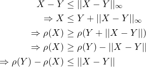
Note that the first switch from ![]() to
to ![]() is caused by applying the monetary measure and its monotonicity property. Afterwards the cash invariance property is applied and the inequality is multiplied by
is caused by applying the monetary measure and its monotonicity property. Afterwards the cash invariance property is applied and the inequality is multiplied by ![]() such that the inequality sign changes again.
such that the inequality sign changes again.
Repeating the same argument on ![]() yields
yields ![]() and thus the assertion.
and thus the assertion.
![]()
Lemma 4.1 implies the existence of an unique extension of ![]() on
on ![]() . Therefore, we can define the expectation operator
. Therefore, we can define the expectation operator ![]() with respect to a finitely additive measure
with respect to a finitely additive measure ![]() of total mass 1. We are going to study this connection in the upcoming Part II of this series in detail.
of total mass 1. We are going to study this connection in the upcoming Part II of this series in detail.
Notice that a coherent risk measure corresponds to the upper expectations.
Popular Risk Measures
Let us start with a very easy example and then introduce the undoubtedly most famous monetary measure of risk – the value at risk measure.
Worst-Case Risk Measure
The following risk measure just takes the worst case for a financial position.
Definition 5.1 (Worst-Case Risk Measure)
The worst-case risk measure ![]() is defined by
is defined by
![]()
![]()
The value ![]() is the least upper bound for the potential net present value, which can occur in any scenario. That is, the infimum is applied as we need to ensure the worst case of all loses across all scenarios
is the least upper bound for the potential net present value, which can occur in any scenario. That is, the infimum is applied as we need to ensure the worst case of all loses across all scenarios ![]() is taken. Finally, all profits/losses are multiplied by -1 since we want to turn the losses, that are denoted with negative numbers, to positive risk figures (to match the convention).
is taken. Finally, all profits/losses are multiplied by -1 since we want to turn the losses, that are denoted with negative numbers, to positive risk figures (to match the convention).
The corresponding acceptance set equals

Given that ![]() is a function (vector) space, the acceptance set
is a function (vector) space, the acceptance set ![]() is given by a convex cone of all non-negative functions – refer to (d) of Example 3.3.
is given by a convex cone of all non-negative functions – refer to (d) of Example 3.3.
According to (e) of Proposition 4.2, ![]() is a coherent measure of risk. Let us check the properties anyway:
is a coherent measure of risk. Let us check the properties anyway:
The function ![]() is monotone: if
is monotone: if ![]() dominates
dominates ![]() , then
, then ![]() for all
for all ![]() and we can conclude that
and we can conclude that
![]()
The cash translation invariance follows also from the rules of the infimum:
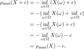
Hence, it is a monetary measure of risk. The risk measure ![]() is also positively homogenous according to the properties of infimum on the real line.
is also positively homogenous according to the properties of infimum on the real line.
By definition, it is the most conservative measure of risk in the sense that any normalized monetary risk measure ![]() on
on ![]() satisfies
satisfies
![]()
for all ![]() .
.
Note that ![]() can be represented in the form
can be represented in the form
![]()
where ![]() is the class of all probability measures on
is the class of all probability measures on ![]() .
.
Value at Risk
Up to now, we have only worked on function spaces, not assuming any probability measure. Value at risk (VaR) subsumes the concept of maximum loss that a financial position may experience over the risk horizon ![]() up to an assigned level of confidence
up to an assigned level of confidence ![]() . We therefore assume that a probability measure
. We therefore assume that a probability measure ![]() on
on ![]() models our financial positions
models our financial positions ![]() with cumulative distribution function
with cumulative distribution function ![]() . Positive values of
. Positive values of ![]() denote profits while negative values denote losses accrued over
denote profits while negative values denote losses accrued over ![]() .
. ![]() is the basic set and
is the basic set and ![]() the corresponding
the corresponding ![]() -algebra.
-algebra.
In plain English, the “value at risk” of a random variable ![]() on
on ![]() is a real number
is a real number ![]() , such that the probability of a loss (i.e.
, such that the probability of a loss (i.e. ![]() ) is bounded by a given level
) is bounded by a given level ![]() . Usually
. Usually ![]() is set to
is set to ![]() . That is,
. That is,
![]()
Let us define the corresponding monetary risk measure.
Definition 5.2 (Value at Risk)
The value at risk (measure) ![]() at level
at level ![]() is defined by
is defined by
![Rendered by QuickLaTeX.com \begin{align*} \rho_{\text{VaR}_{\lambda}}(X)&:=\inf_{\omega \in \Omega}\{c\in \mathbb{R} | \ P[X(\omega)+c<0] \leq \lambda \}\\ &= F^{-1}_X(\lambda), \end{align*}](https://www.deep-mind.org/wp-content/ql-cache/quicklatex.com-1f9cf4db6ba178138d118ca87c71f97d_l3.png)
which refers to a quantile of the loss distribution of ![]() .
.
![]()
Given that the VaR is a loss measure, the quantile needs to be chosen accordingly. On the one hand, if losses are denoted by negative figures, then we need to restrict events such as ![]() by requiring
by requiring ![]() . This is exactly the situation that we have here according to the definitions of section 2.
. This is exactly the situation that we have here according to the definitions of section 2.
On the other hand, if losses are denoted by positive figures, events like ![]() need to be rstricted by requiring
need to be rstricted by requiring ![]() .
.
Value at risk is the smallest amount of capital ![]() which, if added to
which, if added to ![]() as a risk-free investment, needs to keep the probability of a negative outcome below the level
as a risk-free investment, needs to keep the probability of a negative outcome below the level ![]() . Let us illustrate that using a simple example.
. Let us illustrate that using a simple example.
If, for instance, cash of ![]() is added to a profit-and-loss profile, the entire profile is shifted to the right by
is added to a profit-and-loss profile, the entire profile is shifted to the right by ![]() . The corresponding risk distribution, however, is shifted by
. The corresponding risk distribution, however, is shifted by ![]() to the left as sketched in the following graph.
to the left as sketched in the following graph.
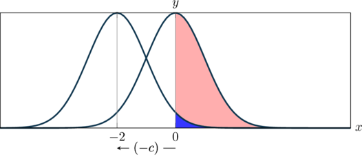
By definition or convention, risk is reflected by positive and chance by negative figures.
Example 5.1 (VaR of Risk-Free Investment)
Let us calculate the value at risk of a risk-free investment ![]() . We assume that holding an amount of cash
. We assume that holding an amount of cash ![]() is risk-free, for instance. If we add the deterministic pay-off profile to the definition of the value at risk, we receive the following:
is risk-free, for instance. If we add the deterministic pay-off profile to the definition of the value at risk, we receive the following:
![Rendered by QuickLaTeX.com \begin{align*} &\rho_{\text{VaR}}(X=d)\\ &=\inf_{\omega \in \Omega}\{c\in \mathbb{R} | \ P[X+c<0] \leq \lambda \} \end{align*}](https://www.deep-mind.org/wp-content/ql-cache/quicklatex.com-52648bdb25c20a4a2bd49dfdadc6015f_l3.png)
We need to figure when the condition ![]() holds true for
holds true for ![]() . Thereby we need to consider that the random variable is deterministic such that we either fulfill the condition or not. If we set
. Thereby we need to consider that the random variable is deterministic such that we either fulfill the condition or not. If we set ![]() to a value smaller or equal than
to a value smaller or equal than ![]() , i.e.
, i.e. ![]() , then the condition
, then the condition ![]() holds true for all
holds true for all ![]() , such that we have
, such that we have ![]() . Thus,
. Thus, ![]() with
with ![]() cannot be true.
cannot be true.

It therefore turns out that ![]() is fulfilled if
is fulfilled if ![]() . Taking the infimum
. Taking the infimum ![]() results in
results in ![]() .
.
![]()
If ![]() dominates
dominates ![]() , i.e.
, i.e. ![]() for all
for all ![]() , then the financial position
, then the financial position ![]() provides more return than
provides more return than ![]() , no matter what scenarios occurs. Hence, for a fixed
, no matter what scenarios occurs. Hence, for a fixed ![]() , an arbitrary
, an arbitrary ![]() and
and ![]() , we conclude the monotonicity of the value at risk:
, we conclude the monotonicity of the value at risk:
![Rendered by QuickLaTeX.com \begin{align*} &\qquad X(\omega) \leq Y(\omega) \quad \forall \omega\in \Omega \\ &\Rightarrow \{\omega | X(\omega) < -c\} \supseteq \{\omega | Y(\omega) < -c\} \\ &\Rightarrow \{c | P[X+c < 0 ] \leq \lambda \} \supseteq \\ &\qquad \{c | P[Y+c < 0] \leq \lambda \} \\ &\Rightarrow \rho_{\text{VaR}}(X) \geq \rho_{\text{VaR}}(Y). \end{align*}](https://www.deep-mind.org/wp-content/ql-cache/quicklatex.com-d822c6b11fa34af227f9003b16b1331e_l3.png)
Since the profit and loss profile of ![]() is always worse than this of
is always worse than this of ![]() , we need to add more cash to cover potential losses of
, we need to add more cash to cover potential losses of ![]() compared to
compared to ![]() . Hence, the set
. Hence, the set ![]() is a superset to
is a superset to ![]() , which ultimately results in the asserted inequality that proves the monotonicity.
, which ultimately results in the asserted inequality that proves the monotonicity.
To prove the cash translation invariance, we recall Example 5.1 where we have shown that ![]() for an amount of cash
for an amount of cash ![]() . If
. If ![]() , then the cash translation invariance follows via
, then the cash translation invariance follows via
![Rendered by QuickLaTeX.com \begin{align*} &\rho_{\text{VaR}}(Y+d) \\ &=\inf_{\omega \in \Omega}\{c=(c_X+c_d) \in \mathbb{R} | \ P[Y+c<0] \leq \lambda \}\\ &=\inf_{\omega \in \Omega}\{(c_X+c_d)\in \mathbb{R} | \ P[X+(c_X+c_d)<0] \leq \lambda \}\\ &=\inf_{\omega \in \Omega}\{c_X \in \mathbb{R} | \ P[X+c_X<0] \leq \lambda \} \\ &+\inf_{\omega \in \Omega}\{c_d\in \mathbb{R} | \ P[d+c_d<0] \leq \lambda \} \\ &=\rho_{\text{VaR}}(X+c_X)-d. \end{align*}](https://www.deep-mind.org/wp-content/ql-cache/quicklatex.com-dce75b5c3c93831ac0a0c2f35ca63695_l3.png)
Thereby, consider Example 5.1 as well as the the rules of the infimum.
Hence, the following proposition follows.
Proposition 5.1 (VaR is a Monetary Risk Measure)
Cash translation invariance, monotonicity, and positive homogenity hold for a VaR measure. That is, VaR is a monetary measure of risk.
![]()
The risk measure ![]() is, however, not subadditive as the following example shows.
is, however, not subadditive as the following example shows.
Example 5.2 (VaR not subadditive)
Consider an investment into two defaultable zero bonds ![]() and
and ![]() , each with return
, each with return ![]() ,
, ![]() , where
, where ![]() is the return of a ‘riskless’ investment. We furthermore assume that both bonds default mutually independent from each other, that both bonds have the same default probability of
is the return of a ‘riskless’ investment. We furthermore assume that both bonds default mutually independent from each other, that both bonds have the same default probability of ![]() and. Refer to Binomial- and Poisson-Mixture Models for further details.
and. Refer to Binomial- and Poisson-Mixture Models for further details.
The discounted net gain of an investment ![]() in one of the two bonds is given by
in one of the two bonds is given by

That is, we assume a loss given default of ![]() for all
for all ![]() such that the investment
such that the investment ![]() will be lost completely in case of a default. According to Proposition 4.1 the Infimum of
will be lost completely in case of a default. According to Proposition 4.1 the Infimum of ![]() such that
such that ![]() equals the risk. Hence, for both bonds, we have
equals the risk. Hence, for both bonds, we have
![Rendered by QuickLaTeX.com \begin{align*} &P\left[ X_i + \left( -\frac{N (\tilde{r}-r)}{1+r} \right) < 0 \right] \\ & = P[\text{Default of } X_i ] \\ & = \text{PD}. \end{align*}](https://www.deep-mind.org/wp-content/ql-cache/quicklatex.com-8553da5a7301c07df30a8b454d4d9e56_l3.png)
This means that both positions ![]() are acceptable if we add
are acceptable if we add ![]() for
for ![]() cash to each financial position (i.e. portfolio). That is,
cash to each financial position (i.e. portfolio). That is, ![]() and
and ![]() .
.
Now, consider the financial position ![]() , which comprises the first two portfolios but equally weighted by
, which comprises the first two portfolios but equally weighted by ![]() . According to (4) of Binomial- and Poisson-Mixture Models, the probability that
. According to (4) of Binomial- and Poisson-Mixture Models, the probability that ![]() out of the
out of the ![]() bonds default can be calculated as follows:
bonds default can be calculated as follows:
![]()
Employing the same argument as above, we can derive the risk as follows.
![Rendered by QuickLaTeX.com \begin{align*} &P\left[ Y + \left( -\frac{N (\tilde{r}-r)}{1+r} \right) < 0 \right] \\ & = P[\text{Default of } X_1 \text{ or } X_2 ] \\ & = \text{PD}^2. \end{align*}](https://www.deep-mind.org/wp-content/ql-cache/quicklatex.com-a6f7315bbe7164ac819440a7d3b9622d_l3.png)
![]()
Another weakness of the VaR is that it does not properly reflect unlikely but catastrophic risks in the relevant tail of the distribution. A natural remedy for not considering unlikely loss events would be to consider the average VaR values beyond some confidence level. This leads us to a risk measure called Expected Shortfall or Average Value at Risk.
Expected Shortfall
The risk measure for market risk according to the Fundamental Review of the Trading Book is the Expected Shortfall (ES). It overcomes the main weaknesses of the VaR.
Definition 5.3 (Expected Shortfall)
The Expected Shortfall (ES) at level ![]() of a position
of a position ![]() is given by
is given by
![]()
The ES is also called Average VaR and Conditional VaR.
![]()
The ES inherits its properties from the VaR as the integral function is even linear. For the proof that the ES is sublinear we refer to the Paper “Seven Proofs for the Subadditivity of Expected Shortfall” by Embrechts and Wang.
Literature
[1]
[2]
[3]
[4]
[5]


