The Capability of Neural Networks as General Function Approximators
Introduction
Artificial Intelligence has become very present in the media in the last couple of years. At the end of 2022, ChatGPT has captured the world’s attention, showing at least a hundred million users around the globe the extraordinary potential of large language models. Large language models such as LLaMA, Bard and ChatGPT mimic intelligent behavior equivalent to, or indistinguishable from, that of a human in specific areas (i.e., Imitation Game or Turing Test). Stephen Wolfram has written an article about how ChatGPT works.
Year-end 2022 might therefore be a watershed moment for human mankind since Artificial Intelligence has now the potential to change the way how humans think and work. Recall further achievements such as
- predicting the 3D models of protein structures,
- predicting chaotic systems, and
- mastering the game of Go.
All these achievements have one thing in common – they are build on a model using an Artificial Neural Networks (ANN).
But what is an ANN?
An ANN is a logical system inspired by biological neural networks that constitute a processing of information just like in brains. I recommend the following video “But what is a neural network?” by 3blue1brown as it builds up an illustrative interpretation of the mechanics of neural nets in a very thorough and concise fashion.
The main objective of this post is to answer the more fundamental question
- Why are Artificial Neural Networks so powerful in solving specific tasks?
The actual answer is quite plain and it may even be a bit disappointing. It ultimately comes down to mathematics but don’t be scared off, we will take each step together.
ANN are very good function approximators provided that big data of the corresponding domain is available. Almost all practical problems such as playing a game of Go or mimic intelligent behavior can be represented by mathematical functions.
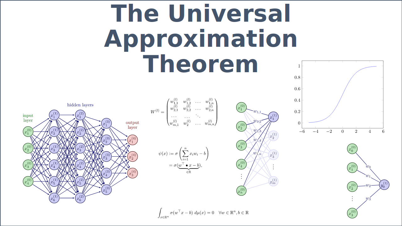
The corresponding theorem that formulates this basic idea of approximation is called Universal Approximation Theorem. It is a fundamental result in the field of ANN, which states that certain types of neural network can approximate certain function to any desired degree of accuracy. This theorem suggest that a neural network is capable of learning complex patterns and relationships in data as long as certain conditions are fulfilled.
The Universal Approximation Theorem is the root-cause why ANN are so successful and capable in solving a wide range of problems in machine learning and other fields.
Before we actually dive into this very important but also specific theorem, let us first consider the architecture of neural nets. Afterwards, we are going to delve into the role of functions for ANN. Then we will outline and prove one version of the Universal Approximation Theorem and refer to other versions. Apart from the theory, we will also provide simple Python code which will approximate specific mathematical functions to showcase the theorem.
Structure of Neural Networks
We are going to introduce the basics structural or architectural aspects of ANNs. It will turn out that this knowledge is helpful in understanding the different versions of the Universal Approximation Theorem.
Layers
ANNs consist of interconnected nodes –called neurons, nodes or units– which process and transmit data through a series of connections. The output of one neuron might be fed as an input to a subsequent neuron. It can therefore be represented by a directed graph, i.e. a digraph, as shown in Fig. 1.

Figure 1: Typical structure of a fully connected ANN comprising one input, several hidden as well as one output layer.
The direction within the digraph represents the information flow. Each arrow from a source to a target neuron indicates that the output value of the source is used as an input value to the target.
In this post, we restrict ourselves to so-called Feedforward Neural Networks, where only specific digraphs are of interest. For instance, loops or multiple edges are not desirable in this architecture.
The generic layered architecture (of a neural network) can be divided into three different types:
- Input layer
Receives input data and passes it on to the hidden layers without any real computation. A neuron in the input layer can be considered as the identify function, though. - Hidden layer
These are the layers that usually perform the majority of the computation in the network. There can be one or more hidden layers in an ANN, and the number of hidden layers and the number of neurons in each hidden layer can vary widely depending on the complexity of the problem being solved. - Output layer
Receives the output from the hidden layers, conducts the final computation, and produces the ultimate output of the entire network.
The input layer usually corresponds with the data at hand. For instance, if we want to train a neural network to recognize handwritten digits employing the MNIST database, the input layer might consist of 784 = 28 ![]() 28 input neurons simply because each picture has a resolution of 28 times 28. An input layer does not have weights or biases assigned to it.
28 input neurons simply because each picture has a resolution of 28 times 28. An input layer does not have weights or biases assigned to it.
The hidden layers perform the majority of the computation. The simpler the hidden layers of a neural network are, the less complex problems can be solved by the corresponding ANN. Each hidden layer learns different aspects about the data by minimizing an assigned loss/cost function. Within these layers the ‘black magic’ happens.
The size of the output layer usually corresponds with the intended result that we try to achieve. In the last layer, the final computations are performed based on the result of the hidden layers. The result of this computation is the final output of the network. For example, in the MNIST classification problem of recognizing handwritten digits, the output layer might produce some sort of (probability) distribution over the set of digits 0, 1, ![]() , 9, with the class with the highest ‘probability’ being the predicted class.
, 9, with the class with the highest ‘probability’ being the predicted class.
The architecture of an ANN along with its activation function is one of the most important factors that enables the network to approximate even complex, non-linear relationships. Activation functions are explained further down.
Types
We are going to study types of ANN to further support the understanding of the Universal Approximation Theorem. Note that this is neither intended as a complete list of ANN nor as a full explanation of the treated types.
McCulloch & Pitts Neurons
The first conceptual or mathematical model of a (biological) neuron was proposed by McCulloch and Pitts in their paper ‘A logical calculus of the ideas immanent in nervous activity‘ in 1943. The McCulloch-Pitts unit was primarily used as a theoretical tool to explore the idea, that the brain could be modeled as a large collection of simple processing elements. This logical system was not trainable since it only could be configured with fixed weights and it was not able to model complex relationships.
Rosenblatt Perceptron
In 1958 Frank Rosenblatt, an American psychologist, proposed the perceptron model, a type of ANN that is a more general computational model than McCulloch-Pitts units. The book Principles of Neurodynamics by F. Rosenblatt summarizes his work on perceptrons.
A perceptron consists of one or more input values that are connected to via corresponding weights to a single output neuron. The input values are multiplied by a set of weights and summed. This sum is then passed through an activation function, usually a step function, which produces a binary output (0 or 1). The goal of training a perceptron is to adjust the weights in such a way that the perceptron produces the correct output for a given set of input values.
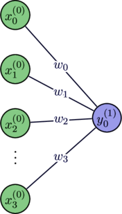
Figure 2: Sketch of a typical Perceptron ANN
Given its restricted output (0 or 1), the perceptron can only be used for binary classification problems. The single layer architecture as well as the use of a (linear) step function as an activation function restricts its successful use further to linear problems.
The following video provides some insights to the early days in machine learning.
The training process for a perceptron is done through a supervised learning method called the Perceptron Learning Algorithm. This algorithm adjusts the weights based on the difference between the desired output and the actual output (error) produced by the perceptron. Since learning algorithms are, however, not in scope of this post we refer to the following video Pattern Recognition Episode 19 Roseblatt Perceptron by Andreas Maier.
It’s important to note that a single-layer perceptron is not able to model complex non-linear decision boundaries. Refer to section Perceptron, where Example 4.1 shows that even a very simple Boolean function –such as the XOR function– cannot be approximated by this kind of simple ANN.
Multi-Layer Feed-Forward Neural Networks
Multi-Layer Feed-Forward Neural Networks are ANN with at least one hidden layer to model more complex relations. Each neuron in one layer has directed connections to the neurons of the subsequent layer. Note that the term multi-layer perceptron is sometimes used loosely to refer to any feed-forward neural network, while in other cases it is restricted to specific ones such as ANN with specific activation functions or trained by the perceptron algorithm.
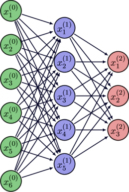
Figure 3: Sketch of a simple multi-layer or shallow ANN
The neurons of a Multi-Layer Neural Network are typically organized into the above defined three types of layers, i.e. there is at least one hidden layer.
In this post, we consider an ANN with one hidden layer to be a shallow. There is no general rule for how many layers an ANN must have to be considered deep, and the definition can vary depending on the specific application or context.
Deep ANNs are designed to learn increasingly complex representations of input data as they progress through multiple layers. By using multiple layers, deep ANNs can potentially capture more complex relationships between inputs and outputs, which may be useful for tasks such as image recognition, speech recognition and natural language processing. For instance, ChatGPT has 175 billion parameters and consists of 96 layers (acc. to ChatGPT).
In this post, however, we will focus on simpler ANN such as shallow ANN. By just adding one hidden layer, the approximation power will be drastically improved as we will see in section Shallow Feed-Forward ANN.
Neural Networks and Functions
McCulloch and Pitts proposed that the biological neurons in the brain can be modeled as simple logical functions that take inputs and produce weighted outputs. They proposed that these logical functions can perform more complex computations if connected together in a network and they suggested that the neurons in the brain work together in a similar way. This exact idea formed the basis for the development of the first ANN, which are also modeled as networks of interconnected simple processing elements, or artificial neurons, that work together to perform more complex computations.
In this section, we will follow that path and first study how a single neuron can be represented by a function. Then we extend this idea to layers (, i.e., a collection of nodes) and lastly to the entire ANN. We will restrict ourselves to what is needed for a proper understanding of the Universal Approximation Theorem. We also explain what role so-called activation functions play.
Apparently, it is of utter importance to understand what a function actually is. Hence, let us quickly recall how a mathematical function is defined.

Figure 4: Illustration of the definition of a function.
In Fig. 4, set ![]() and
and ![]() are the domain and the range of the function
are the domain and the range of the function ![]() , respectively. The function
, respectively. The function ![]() maps every element
maps every element ![]() of the domain to exactly one element
of the domain to exactly one element ![]() of its range. Not all elements of the range need to have a counterpart in the domain but every element of the domain needs to be mapped to a function value in the range. Note that a functional is a certain type of function, where the range is
of its range. Not all elements of the range need to have a counterpart in the domain but every element of the domain needs to be mapped to a function value in the range. Note that a functional is a certain type of function, where the range is ![]() .
.
Neurons as Functionals
A meaningful neuron needs to have
- input values
 along with corresponding
 - weight values
 . In addition,
 - each neuron (of a hidden and output layer) has its own bias value
 .
.
If we consider the inputs ![]() as well as the corresponding weights
as well as the corresponding weights ![]() as two vectors of a
as two vectors of a ![]() -dimensional vector space
-dimensional vector space ![]() , and
, and ![]() as a scalar (i.e. a real value), we can represent this single neuron as a functional
as a scalar (i.e. a real value), we can represent this single neuron as a functional ![]() , defined by
, defined by
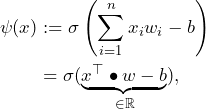
where ![]() is an activation function. The weighted sum can also be denoted as dot / inner product of the two vectors, that is,
is an activation function. The weighted sum can also be denoted as dot / inner product of the two vectors, that is, ![]() =
= ![]() .
.
Note that ![]() as well as
as well as ![]() are considered to be constants that are only changed during the training of an ANN. We therefore suppress those constants in the notation of the function. The input vector
are considered to be constants that are only changed during the training of an ANN. We therefore suppress those constants in the notation of the function. The input vector ![]() are given or generated by previous neurons. Activation functions are explained in the next section, however, be aware that activation functions are –in general– not linear. They actually need to be non-linear in specific situations.
are given or generated by previous neurons. Activation functions are explained in the next section, however, be aware that activation functions are –in general– not linear. They actually need to be non-linear in specific situations.
Each neuron –of a hidden and an output layer– compute the weighted sum of inputs and weights, then deduct the bias and execute an activation function. The weighted sum is a linear function but the activation function can be of non-linear type.
Given that we intend to extend the function notation of neurons to entire layers or even entire ANN, we also need to consider the sources and targets of the function parameters. Fig. 5 will support the understanding.
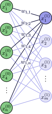
Figure 5: Extract of an ANN to illustrate notation.
Given that the output of one neuron might be the input to another, it is necessary to denote the number of the layer to all inputs and biases.
The weights can be interpreted as the (directed) connections between neurons of two adjacent layers as sketched above. Hence, the neuron ![]() –as sketched in Fig. 5– can therefore be represented by its corresponding functional
–as sketched in Fig. 5– can therefore be represented by its corresponding functional ![]() denoted by
denoted by

If we generalize this notation, we receive

Please also refer to Fig. 5 for an illustration of the notation. It is important to realize that the weights ![]() connect neurons between two adjacent layers
connect neurons between two adjacent layers ![]() and
and ![]() and that
and that ![]() and
and ![]() are running variables for the number of neurons in layer
are running variables for the number of neurons in layer ![]() and
and ![]() , respectively.
, respectively.
We can therefore state that neurons can be represented by multiple composition of affine functions and nonlinear activation functions. Before we move on to extend that idea to entire layers of ANN, let us first have a close look at activation functions.
Activation Function
An activation function is a functional that is applied to an intermediary output of a neuron as outlined in section Neurons as Functionals. It determines the final output of the neuron. Activation functions are an important element of neural networks because they support the network to model complex nonlinear relationships between the input and output data. However, activation functions are not the only parts of an ANN that enables it to approximate non-linear relationships.
The following class of activation function will play an important role in proving the Universal Approximation Theorem.
Definition 3.1: (Sigmoidal Activation Function)
An activation function ![]() is called sigmoidal if
is called sigmoidal if

![]()
The following types are the most commonly used activation functions. All of these examples, except the ReLU, are sigmoidal. This can be proven formally by simply applying the definition and considering the limits.
Sigmoid function
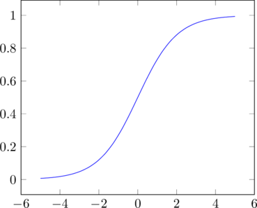
The sigmoid function ![]() maps any real-valued number to a value between 0 and 1. It is often used as an activation function in the output layer of a binary classification neural network and is defined as follows.
maps any real-valued number to a value between 0 and 1. It is often used as an activation function in the output layer of a binary classification neural network and is defined as follows.
![]()
The graph of this function can be sketched as follows.
Hyperbolic Tangent function
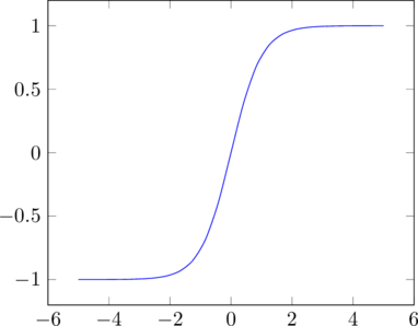
The tanh function ![]() maps any real-valued number to a value between -1 and 1. It is similar to the sigmoid function, but it is centered at 0 and a different domain. The exact definition is as follows.
maps any real-valued number to a value between -1 and 1. It is similar to the sigmoid function, but it is centered at 0 and a different domain. The exact definition is as follows.
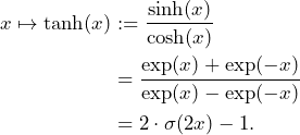
The graph of this function can be sketched as follows.
ReLU function
The Rectified Linear Unit (ReLU) function maps any negative input to 0 and any positive input to itself. It is often used as an activation function in the hidden layers of a neural network. The exact definition is as follows.
![]()
where ![]() is the absolute value function. The graph of this function can be sketched as follows.
is the absolute value function. The graph of this function can be sketched as follows.
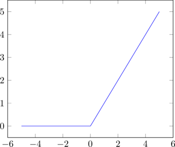
The ReLU function, however, is not sigmoidal since ![]() .
.
Another important feature of an activation function is whether it can be considered as discriminatory.
Definition 3.2 (Discriminatory Activation Function)
Let ![]() be a measure on
be a measure on ![]() . An activation function
. An activation function ![]() is then called discriminatory, if
is then called discriminatory, if
![]()
implies that the measure ![]() is the zero measure (i.e.
is the zero measure (i.e. ![]() ).
).
![]()
This definition therefore tells us that the activation function cannot distinct between two indistinguishable sets of points of the domain. In this context, a set of points of the domain is considered equal if they equal almost everywhere with respect to the measure ![]() . That is, they equal under the measure
. That is, they equal under the measure ![]() with the exception of zero sets.
with the exception of zero sets.
Hence, a discriminatory activation function is one that can be used to define decision boundaries between different sets of inputs (almost everywhere wrt. ![]() ). By composing such functions in a multi-layer feed-forward network, we can construct complex decision boundaries that allow us to approximate arbitrary functions.
). By composing such functions in a multi-layer feed-forward network, we can construct complex decision boundaries that allow us to approximate arbitrary functions.
Let us now generalize the relationship between a neuron and a functional to a collection of neurons also known as layer.
Layers as Functions
Before we consider the situation for an entire layer, let us recap what we have derived in the section Neurons as Functionals.
If ![]() stimuli / inputs
stimuli / inputs ![]() of the input layer are received by one neuron
of the input layer are received by one neuron ![]() of the first hidden layer, each of the stimulus / input
of the first hidden layer, each of the stimulus / input ![]() will be multiplied with an associated weight
will be multiplied with an associated weight ![]() . Think about what the indices of the weights actually mean– the superscript indicates the number of the layer while the subscripts indicate the receiving neuron as well as the number of the input values.
. Think about what the indices of the weights actually mean– the superscript indicates the number of the layer while the subscripts indicate the receiving neuron as well as the number of the input values.
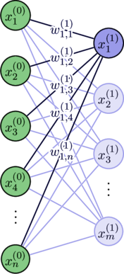
Figure 6: ANN comprising input values, weights, and the first hidden layer.
After the weighted sum of all stimuli / inputs has been calculated, the bias ![]() is deducted and the resulting real figure is fed into an activation function. The final output of the neuron
is deducted and the resulting real figure is fed into an activation function. The final output of the neuron ![]() might then be fed as input to another neuron of the next layer.
might then be fed as input to another neuron of the next layer.
Fig. 6 shows the relationship between the neuron ![]() , the corresponding input values
, the corresponding input values ![]() , and the weights
, and the weights ![]() . Other neurons of the same layer such as
. Other neurons of the same layer such as ![]() might have the same input vector
might have the same input vector ![]() , but the weights
, but the weights ![]() usually differ.
usually differ.
By collecting the weight vector of each node for the entire target layer ![]() , we can create a weight matrix
, we can create a weight matrix ![]() , that contains these weight vectors row-wise.
, that contains these weight vectors row-wise.
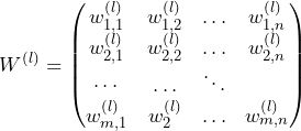
Note that the weight matrix ![]() contains the weights of the connections between the layer
contains the weights of the connections between the layer ![]() and
and ![]() .
.
We also need to put all the biases of the neurons of layer ![]() together, such that we get a
together, such that we get a ![]() -dimensional vector
-dimensional vector ![]() .
.
Now, we can easily define a multivariate function ![]() by combining the functionals of each neuron within the relevant layer.
by combining the functionals of each neuron within the relevant layer.
To this end, it is convenient to use a matrix multiplication of a ![]() weight matrix with a
weight matrix with a ![]() input vector resulting in a
input vector resulting in a ![]() output vector which is added to the negative of a
output vector which is added to the negative of a ![]() bias vector. Then, an activation function is applied element-wise to each of the
bias vector. Then, an activation function is applied element-wise to each of the ![]() entries of the vector. This can be denoted by
entries of the vector. This can be denoted by
![]()
The final ![]() output vector is just an ordered collection of the outputs of the single neurons / functionals of the target layer
output vector is just an ordered collection of the outputs of the single neurons / functionals of the target layer ![]() . The big advantage of such a representation in matrix form is that it can be leveraged by parallel computation using a GPU, for instance.
. The big advantage of such a representation in matrix form is that it can be leveraged by parallel computation using a GPU, for instance.
Example 3.1 (Linear and Polynomial Activation Functions)
Let us consider a fully connected ANN with one hidden layer and an output layer with a single neuron, that can be represented with the functional
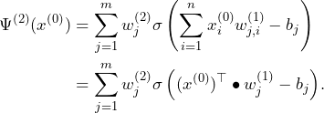
That is, the ANN consists of one input layer, comprising ![]() , one hidden layer with
, one hidden layer with ![]() neurons, and one output layer with one neuron with value
neurons, and one output layer with one neuron with value ![]() . By simplifying the notation using
. By simplifying the notation using ![]() instead of
instead of ![]() , we can conclude:
, we can conclude:
- If
 equals the identity function, then
  , which is an affine linear function.
 - If
 is a linear activation function then
  is an affine linear function.
 - If
 is a polynomial of degree
  , then the function
  with
with  hidden layers is a polynomial of degree at most
  .
.
![]()
At last, we could also define a function ![]() that consist of functions
that consist of functions ![]() where
where ![]() is a running variable for all hidden and output layers. Thereby, the domain of
is a running variable for all hidden and output layers. Thereby, the domain of ![]() corresponds with its input while the range with its output vector.
corresponds with its input while the range with its output vector.
We can summarize that ANN, or layers of ANN, can be represented by multiple compositions of affine functions and nonlinear activation functions.
Universal Approximation Theorem
We start off the core chapter with a section about a perceptron, which is the simplest kind of an ANN and actually a counterexample of an universal approximator. It lacks to solve even simple problems as we will see in Example 4.1.
Afterwards, we are studying the shallow feed-forward ANN and prove that these networks are universal approximators. At last, we also provide an overview on different versions of the Universal Approximation Theorem based on different types of ANN.
Perceptron
The perceptron is limited by its architecture. A single-layer perceptron can only represent linear functions, and thus it can only classify linearly separable data. For example, it cannot learn to recognize a circle, as it’s a non-linear boundary.
In other words, it can only solve classification problems where the boundary between the classes is a hyperplane (line in 2D, plane in 3D, etc) . It fails to approximate any non-linear function, which are common in real-world data.
Example 4.1: (Boolean Functions)
Let us now study the Boolean function AND, OR and XOR.
A function is called perceptron-computable if the points, whose function value is False (i.e. 0), can be separated from the points whose function values are True (i.e. 1) using a line (i.e. a hyperplane). If green and red indicate the function value 1 and 0, respectively, we can visualize the truth table in the plane ![]() of these Boolean functions.
of these Boolean functions.
AND function of two variables
| 1 | 1 | 1 |
| 1 | 0 | 0 |
| 0 | 1 | 0 |
| 0 | 0 | 0 |
Recall, if green and red indicate the function value 1 and 0, respectively, we can visualize the truth table in the plane ![]() of the AND function as follows.
of the AND function as follows.

Apparently, it is possible to model the AND function correctly using the perceptron. A perceptron can only model a linear function that outputs two states 0 or 1. A line that separates the two output states correctly is illustrated in the graph above. Note that this line is a hyperplane in ![]() and there are infinite many correct solution to characterize the AND function correctly.
and there are infinite many correct solution to characterize the AND function correctly.
OR function of two variables
| 1 | 1 | 1 |
| 1 | 0 | 1 |
| 0 | 1 | 1 |
| 0 | 0 | 0 |
If we visualize the truth table of the OR function in the plane ![]() , we receive the following.
, we receive the following.
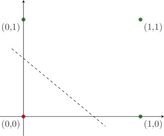
Apparently, it is possible to model the OR function correctly using the perceptron. A line that correctly separates the two output states (1/green and 0/red) is illustrated in the graph above.
XOR function of two variables
| 1 | 1 | 0 |
| 1 | 0 | 1 |
| 0 | 1 | 1 |
| 0 | 0 | 0 |
By comparing the XOR function in ![]() with the AND and the OR function, it is intuitively evident that no line can be approximated by the perceptron to separate the two states 1/green and 0/red. That is, the XOR classification problem is not linearly separable.
with the AND and the OR function, it is intuitively evident that no line can be approximated by the perceptron to separate the two states 1/green and 0/red. That is, the XOR classification problem is not linearly separable.
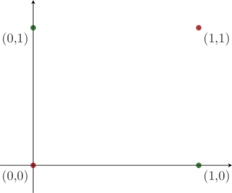
This can also be shown analytically. Let ![]() be two real weights of a perceptron with two inputs, and
be two real weights of a perceptron with two inputs, and ![]() its bias. If the perceptron model reflects the XOR function correclty, the following inequalities need to be fulfilled:
its bias. If the perceptron model reflects the XOR function correclty, the following inequalities need to be fulfilled:

According to the first inequality, the bias ![]() needs to be positive. Similarly, both weights
needs to be positive. Similarly, both weights ![]() and
and ![]() need to be positive. However, then the fourth inequality
need to be positive. However, then the fourth inequality ![]() cannot be true. Note that XOR
cannot be true. Note that XOR![]() . This contradicts our assumption that the XOR function can be modeled correctly by a single-layer perceptron.
. This contradicts our assumption that the XOR function can be modeled correctly by a single-layer perceptron.
![]()
Shallow Feed-Forward ANN
In this section, we investigate the Universal Approximation Theorem as suggested by G. Cybenko in his seminal paper [2] from 1989.
Before we can start, we need to agree on two geometric terms — topology and metric. The topology rules the space in which we approximate and the so-called metric determines how we measure distances. For ![]() , we define
, we define
![]()
and we equip ![]() with the supremum (or uniform) norm of a continuous function
with the supremum (or uniform) norm of a continuous function ![]() denoted by
denoted by ![]() . In general, we use
. In general, we use ![]() to denote the supremum (i.e. kind of maximum) of a function on its domain. The space of finite, signed regular Borel measures on
to denote the supremum (i.e. kind of maximum) of a function on its domain. The space of finite, signed regular Borel measures on ![]() is denoted by
is denoted by ![]() .
.
Let ![]() denote the
denote the ![]() -dimensional unit cube
-dimensional unit cube ![]() .
.
We set ![]() in this chapter.
in this chapter.
The main objective of this section is to investigate whether a shallow ANN such as the following is already an universal approximator.
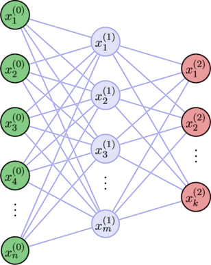
Figure 7: Sketch of a shallow ANN that is an Universal Approximator
But what does it actually mean that an ANN is an universal approximator?
The mathematical toolkit we can use to precisely formulate this idea is given by the field of functional analysis. For further details please refer to [3] and [4].
A set ![]() of functions is called dense in a function space
of functions is called dense in a function space ![]() , if it can approximate any function
, if it can approximate any function ![]() to an arbitrary degree of accuracy. In other words, given any real function
to an arbitrary degree of accuracy. In other words, given any real function ![]() and
and ![]() , there is a real function
, there is a real function ![]() for which
for which
![]()
for all ![]() . The Universal Approximation Theorem therefore claims that at least one neural network exists that can approximate any continuous function on
. The Universal Approximation Theorem therefore claims that at least one neural network exists that can approximate any continuous function on ![]() with arbitrary precision. To this end, the corresponding number of hidden nodes, number of learning iterations, weight parameters and biases need to be adapted individually for the to-be-approximated function
with arbitrary precision. To this end, the corresponding number of hidden nodes, number of learning iterations, weight parameters and biases need to be adapted individually for the to-be-approximated function ![]() .
.
We can therefore reformulate the claim that shallow ANN are universal approximators as follows. Under what conditions is the function
(1) 
dense in the continuous function space ![]() with respect to the supremum norm?
with respect to the supremum norm?
The function ![]() represents a shallow ANN and is therefore of the form (1). The basic idea is that
represents a shallow ANN and is therefore of the form (1). The basic idea is that ![]() can be used to create a sequence of functions that approximates any given function
can be used to create a sequence of functions that approximates any given function ![]() arbitrarily well by changing its parameters like weights and bias (via a training algorithm) or by extending its input values.
arbitrarily well by changing its parameters like weights and bias (via a training algorithm) or by extending its input values.
To this end, let ![]() be the set of functions of the form (1), that can be achieved by any form of training and data. By simplifying the notation to what is really necessary in this context we receive
be the set of functions of the form (1), that can be achieved by any form of training and data. By simplifying the notation to what is really necessary in this context we receive

The following theorem is going to provide an answer.
Universal Approximation Theorem (by Cybenko, [2])
Let ![]() be any continuous discriminatory function. Then finite sums of the form
be any continuous discriminatory function. Then finite sums of the form

are dense in ![]() with respect to the supremum norm.
with respect to the supremum norm.
![]()
Let us first prove that space of functions ![]() generate a linear subspace of the real continuous function vector space. Recall that ANN or layers of ANN are basically multiple compositions of affine functions and (potentially) nonlinear activation functions.
generate a linear subspace of the real continuous function vector space. Recall that ANN or layers of ANN are basically multiple compositions of affine functions and (potentially) nonlinear activation functions.
Proof: To see that ![]() is a linear subspace of
is a linear subspace of ![]() , we only need to realize that
, we only need to realize that ![]() is a linear span of the set
is a linear span of the set
![]()
since ![]() is an arbitrary real number and
is an arbitrary real number and ![]() can be extended (by assumption) to any natural number.
can be extended (by assumption) to any natural number.
![]()
One key tool that we need to use is the so-called Hahn-Banach Theorem, which is an extension theorem for continuous linear functionals defined on a proper linear subspace. It states that we can extend our functional ![]() , that is defined on the linear subspace
, that is defined on the linear subspace ![]() , to a functional
, to a functional ![]() , such that it is still linear and is norm-preserving, i.e.
, such that it is still linear and is norm-preserving, i.e. ![]() .
.
The other functional analysis tool that we need is the Riesz Representation Theorem. This theorem states that any bounded linear functional on the space of compactly supported continuous functions is the same as integration against a measure ![]() .
.
For further details regarding the Hahn-Banach Theorem as well as the Riesz Representation Theorem, we refer to [3] and [4]. There are also good online resources such as the EUDML – Hahn-Banach Theorem and Wolfram Math World – Riesz Representation Theorem.
Now, let us focus on the actual proof of the Universal Approximation Theorem by Cybenko.
Proof: We have already shown that ![]() is a linear subspace of
is a linear subspace of ![]() . We claim that the closure
. We claim that the closure ![]() of
of ![]() is all of
is all of ![]() , i.e., that
, i.e., that ![]() .
.
Assume towards a contradiction that the closure ![]() , then
, then ![]() is a real proper subset of
is a real proper subset of ![]() . By Hahn-Banach theorem, there is a bounded linear functional
. By Hahn-Banach theorem, there is a bounded linear functional ![]() with the property that
with the property that ![]() but
but ![]() . Note that the functional
. Note that the functional ![]() takes continuous functions as input and maps them to scalar of
takes continuous functions as input and maps them to scalar of ![]() .
.
By the Riez Representation Theorem, this bounded linear functional, ![]() , is of the form
, is of the form
![]()
for some ![]() , for all
, for all ![]() . In particular, since
. In particular, since ![]() is in
is in ![]() for all
for all ![]() and
and ![]() , we must have that
, we must have that
![]()
for all ![]() and
and ![]() . However, we assumed that
. However, we assumed that ![]() was discriminatory so that this condition implies that
was discriminatory so that this condition implies that ![]() contradicting the assumption. Hence, the subspace
contradicting the assumption. Hence, the subspace ![]() must be dense in
must be dense in ![]() .
.
![]()
Another interesting perspective on Cybenko’s Theorem is provided by a seminar of the University of Würzburg. The article A visual proof that neural nets can compute any function is provided by Michael Nielsen.
In the next section, we are going to see that there are more than just this version of the Universal Approximation Theorem. These theorems are then based on different ANN architectures.
Other Architectures
The objective of this section is to highlight that for many different architectures of ANN versions of the Universal Approximation Theorem exist. Several groups proved closely related versions of the Universal Approximation Theorem in the 1980s and 1990s.
Apart from Cybenko’s Theorem, the paper ‘Multilayer feedforward networks are universal approximators‘ [5] by Kurt Hornik is another outstanding result. Multilayer feedforward neural networks are ANN with multiple layers. Hornik’s paper, however, uses different techniques (i.e. the Stone-Weierstrass Theorem) to show that an ANN can approximate any Borel measurable function (a more general class of functions that includes discontinuous functions) to any desired degree of accuracy.
Paper [6] by Hornik provides a short overview on the development of the study of approximation capabilities of ANN until 1992 and extends these results further in several ways. The video above by Seigel outlines several parts of the paper [6].
Related questions such as when are deep ANN ‘better than’ shallow ANN in terms of approximation are also interesting and important also from a practical perspective.
The script Neural Network Theory by P. C. Petersen / University of Vienna provides an overview on the different types of Universal Approximation Theorems.
Approximations employing Python/Keras
In this section, we are going to apply our knowledge to approximate standard mathematical functions using ANN. Before we dive in, let us describe the layers of an ANN in a bit more hands-on kind of fashion using the Keras library which is based on Python.
Keras Models and Layers
In most software libraries, you can use layers to build neural networks by creating an instance of the desired layer class and adding it to a so-called model.
A Keras model is a way to organize neural network layers into a logical structure that can be trained and evaluated. Hence, to create a Keras model, we will first need to define the layers of our model. We can then compile the model, specifying the loss function and optimizer to use for training, and finally fit the model to our training data. The following Python code can serve as an example how the layers and therefore the Keras model are defined. Also refer to “Hands-On Machine Learning with Scikit-Learn and TensorFlow” by A. Géron for further details.
import tensorflow as tf
from tensorflow import keras

# Get the data from an online resource
fashion_mnist = keras.datasets.fashion_mnist
(X_train_full, y_train_full), (X_test, y_test) = fashion_mnist.load_data()

# Preprocess data
X_valid, X_train = X_train_full[:5000] / 255.0, X_train_full[5000:] / 255.0
y_valid, y_train = y_train_full[:5000], y_train_full[5000:]
class_names = ["T-shirt/top", "Trouser", "Pullover", "Dress", "Coat", "Sandal", "Shirt", "Sneaker", "Bag", "Ankle boot"]

# Define raw model
model = keras.models.Sequential()

# Define the input layer and add it to the model, i.e., convert each input into a 1-dim. array.
# This layer does not have any parameters.
model.add(keras.layers.Flatten(input_shape=[28, 28]))

# Define the hidden layers and add them to the model
model.add(keras.layers.Dense(300, activation="relu"))
model.add(keras.layers.Dense(100, activation="relu"))

# Define the output layer and add it to the model
model.add(keras.layers.Dense(10, activation="softmax"))

# Check model structure
model.summary()
model.layers

# Compile the model
model.compile(loss='sparse_categorical_crossentropy', optimizer='sgd', metrics=['accuracy'])

# Train the model
model.fit(X_train, y_train, epochs=5)
Example code that illustrates the use of a model and corresponding layers. Refer to chapter 10 of “Hands-On Machine Learning with Scikit-Learn and TensorFlow” by A. Géron
Also refer to the post Different Types of Keras Layers Explained for more details on this topic.
Example Code
Let us now approximate standard functions such as the sine function ![]() , and a specific polynomial function
, and a specific polynomial function ![]() on a specific domain using ANN.
on a specific domain using ANN.
In order to speed the training of these ANN up, we are going to use an Nividia GPU, however, this could also be done using the CPU. Note that the Universal Approximation Theorem doesn’t tell us how we have to approximate such functions in terms of number of nodes of the hidden layer, sample size, number of trainings, etc.
However, the theorem states that we are able to find an arbitrary precise approximation for a certain function using a shallow ANN. We could, of course, also use a deep ANN, this would even lead to better results.
import numpy as np
from tensorflow import keras
from tensorflow.keras import layers
import matplotlib.pyplot as plt


# Generate random training, testing, and validation data
# Training data is used to fit the model, the validation data is used to tune
# the hyperparameters of the model, and the test data is used to evaluate the
# performance of the model on new data
X_train = np.random.uniform(-np.pi, np.pi, 1000)
y_train = np.sin(X_train)

X_test = np.random.uniform(-np.pi, np.pi, 100)
y_test = np.sin(X_test)

X_val = np.random.uniform(-np.pi, np.pi, 100)
y_val = np.sin(X_val)


# Define the layer structure of the neural network
# Input layer which is actually the input of the 1-dim. real Sinus function
input_layer = layers.Input(shape=(1,))
# Hidden layer where the heavy lifting of the approximation of the Sinus function is performed.
# Note that hidden_layer uses the input_layer as input
hidden_layer = layers.Dense(800, activation='sigmoid')(input_layer)
# Output layer which is the result of the 1-dim. real Sinus function.
# Note that output_layer uses the hidden_layer as input
output_layer = layers.Dense(1, activation='linear')(hidden_layer)

# Create the neural network model
model = keras.Model(inputs=input_layer, outputs=output_layer)

# Check model structure
model.summary()
model.layers

# Compile model
model.compile(loss='mean_squared_error', optimizer='adam')

# Fit model to training data with validation
history = model.fit(X_train, y_train, validation_data=(X_val, y_val), epochs=200, verbose=1)

# Evaluate model on test data
loss = model.evaluate(X_test, y_test)

# Generate test data of actual
# and predicted values for plotting
X_test.sort() #sort list since we picked them randomly
y_plot = np.sin(X_test)
y_pred = model.predict(X_test)

# Plot the development of the loss function during training
plt.figure()
plt.plot(history.history['loss'], label='training loss')
plt.plot(history.history['val_loss'], label='validation loss')
plt.legend()
plt.show()


# Plot predicted values and test data
plt.plot(X_test, y_pred, label='Approximation')
plt.plot(X_test, y_plot, label='Actual')
plt.legend()
plt.show()
Example code for the approximation of the sine function using a shallow ANN on the domain ![]()
The result based on a simple shallow ANN is quite good as we can see in the following Fig. 8.
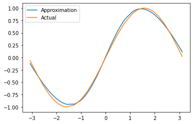
Figure 8: Illustration of an approximation of the sine function by a shallow ANN
Let us now try to approximate a simple polynomial. Even though a shallow ANN is definitely able to approximate such a kind of function, there are many hurdles to overcome. We can see that if we use the code and play around, for instance, if we change the domain.
import numpy as np
from tensorflow import keras
from tensorflow.keras import layers
import matplotlib.pyplot as plt

# Define the polynomial function
def polynomial(x):
    return 2 * x**3 + 3 * x**2 - 5 * x + 2

# Generate random training data
np.random.seed(0)
X_train = np.random.uniform(low=-10, high=10, size=(1000,))
y_train = polynomial(X_train)

# Generate random validation data
X_val = np.random.uniform(low=-10, high=10, size=(100,))
y_val = polynomial(X_val)

# Generate random test data
X_test = np.random.uniform(low=-10, high=10, size=(100,))
y_test = polynomial(X_test)

# Define the model
model = keras.Sequential([
    layers.InputLayer(input_shape=[1]),
    layers.Dense(800, activation='sigmoid'),
    layers.Dense(1)
])


# Compile the model
model.compile(optimizer='adam', loss='mse')

# Train the model
history = model.fit(
    X_train, y_train,
    validation_data=(X_val, y_val),
    epochs=600,
    batch_size=16,
    verbose=1
)


# Evaluate the model on the test data
loss = model.evaluate(X_test, y_test)
print('Test loss:', loss)

# Generate test data of actual
# and predicted values for plotting
X_test.sort() #sort list since we picked them randomly
y_plot = polynomial(X_test)
y_pred = model.predict(X_test)

# Plot the development of the loss function during training
plt.figure()
plt.plot(history.history['loss'], label='training loss')
plt.plot(history.history['val_loss'], label='validation loss')
plt.legend()
plt.show()


# Plot predicted values and test data
plt.plot(X_test, y_pred, label='Approximation')
plt.plot(X_test, y_plot, label='Actual')
plt.legend()
plt.show()
Example code for the approximation of a polynomial using a shallow ANN.
The approximation of the polynomial is also quite good after 600 epochs as we can see in Fig. 9.
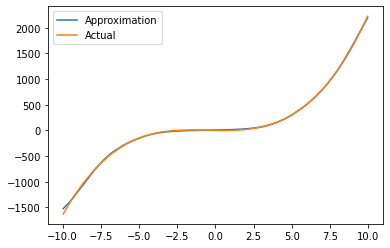
Figure 9: Illustration of an approximation of a polynomial function by a shallow ANN
Note that the example code is by far not as it should be in a serious application. The purpose of this code is just to connect theory and practice and to show where the theory might be able to support.
Conclusion
Cybenko’s Universal Approximation Theorem tells us that Artificial Neural Networks (ANN) are powerful function approximators. Combined with the fact that a mathematical function can represent almost all practical problems, ANN can solve a wide range of complex real-world problems. Neural networks can learn to perform a wide range of tasks, such as classification, prediction, and clustering, by adjusting the weights of the corresponding neurons based on examples from a training dataset. By doing so, it approximates the function that represents a very specific problem.
The more data are at hand, the better the approximation can be. In practice, the big problem is usually the availability and quality of data. There are many problems where data are scarce and inconsistent.
We have seen that the architecture of an ANN is very important. For instance, perceptrons fail to be universal approximator but already shallow ANN are universal approximators. Deep ANN are even better and more efficient in learning specific problems. Cybenko’s Universal Approximation Theorem, however, does not state how fast the approximation is or how many neurons it would require to gain a certain quality of approximation.
The question on how hidden layers should be designed (e.g. the number of the hidden layers, the number of neurons per hidden layer and type of layer), is therefore a question of how the approximation function should be designed to perform best. This translation of the problem might help find better solutions and should therefore be considered when designing an ANN.
According to my understanding, an ANN such as Large Language Models (e.g. ChatGPT) is not really conceive a problem and it can only be applied to one specific problem. This might be different going forward, but right now it doesn’t really matter since Artificial Intelligence is already powerful enough to shape our society.
Literature
For further details and a comprehensive overview on the mathematical modeling of neural networks, we refer to the eBook Neural Networks – A Systematic Introduction by R. Rojas.
[1]
[2]
[3]
[4]
[5]
[6]
Apart from the classical list of literature, the following material is related and might also be of interest for you.
The following video by Prof. P. H. Winston from MIT provides also a great introduction to ANN as function approximators. The entire lecture is worth watching.
If you want to know more about the latter achievement by Google’s DeepMind, there is a movie called AlphaGo – The Movie that tells the story about the development and exiting matches against human professional Go players.

