Convergence ca be defined in many different ways. In this post, we study the most popular way to define convergence by a metric. Note that knowledge about metric spaces is a prerequisite.
In order to define other types of convergence (e.g. point-wise convergence of functions) one needs to extend the following approach based on open sets. This, however, is not in scope of this post.
Limits of a Sequence
In this section, we apply our knowledge about metrics, open and closed sets to limits. We thereby restrict ourselves to the basics of limits. Refer to [1] for further details.
Let ![]() denote a metric space. If the metric is not specified, we assume that the standard Euclidean metric is assigned.
denote a metric space. If the metric is not specified, we assume that the standard Euclidean metric is assigned.
Definition 3.1 (Sequence):
A sequence in ![]() is a function from
is a function from ![]() to
to ![]() by assigning a value
by assigning a value ![]() to each natural number
to each natural number ![]() . The set
. The set ![]()
![]()
![]()
![]() is called sequence of
is called sequence of ![]() . The elements of
. The elements of ![]() are called terms of the sequence.
are called terms of the sequence.
![]()
Sequences in ![]() are called real number sequences. Sequences in
are called real number sequences. Sequences in ![]() ,
, ![]() are called real tuple sequences. Note that latter definition is simply a generalization since number sequences are, of course,
are called real tuple sequences. Note that latter definition is simply a generalization since number sequences are, of course, ![]() -tuple sequences with
-tuple sequences with ![]() .
.
Let ![]() be a
be a ![]() -tuple sequence in
-tuple sequence in ![]() equipped with property
equipped with property ![]() . Property
. Property ![]() holds for almost all terms of
holds for almost all terms of ![]() if there is some
if there is some ![]() such that
such that ![]() is true for infinitely many of the terms
is true for infinitely many of the terms ![]() with
with ![]() .
.
Note that a sequence can be considered as a function with domain ![]() . We need to distinguish this from functions that map sequences to corresponding function values. Latter concept is very closely related to continuity at a point.
. We need to distinguish this from functions that map sequences to corresponding function values. Latter concept is very closely related to continuity at a point.
Sequences are, basically, countably many (![]() – or higher-dimensional) vectors arranged in an ordered set that may or may not exhibit certain patterns.
– or higher-dimensional) vectors arranged in an ordered set that may or may not exhibit certain patterns.
Example 3.1:
a) The sequence ![]() can be written as
can be written as ![]() and is nothing but a function
and is nothing but a function ![]() defined by
defined by ![]() .
.
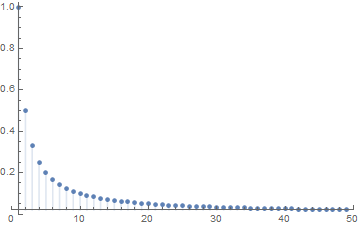
 for
for 
b) Let us now consider the sequence ![]() that can be denoted by
that can be denoted by ![]() . The range of the function only comprises two real figures
. The range of the function only comprises two real figures ![]() .
.
c) Now, let us consider the sequence ![]() . Here, each natural
. Here, each natural ![]() is mapped on itself.
is mapped on itself.
d) Consider ![]() , that can also be written as
, that can also be written as ![]() .
.
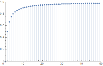

e) Consider the 2-tuple sequence ![]() in
in ![]() .
.
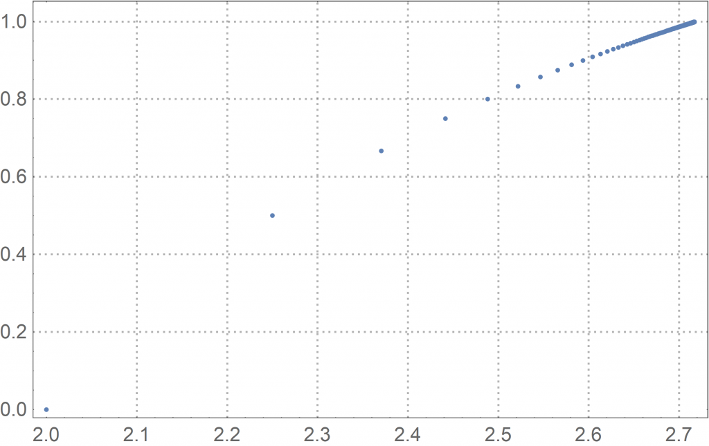
 .
. ![]()
We might think that some of the above examples contain patterns of vectors (e.g. number) that are “getting close” to some other vector (e.g. number). Other sequences may not give us that impression. We are interested in what the long-term behavior of the sequence is:
- What happens for large values of
 ?
? - Does the sequence approach a (real) vector/number?
Note that it is not necessary for a convergent sequence to actually reach its limit. It is only important that the sequence can get arbitrarily close to its limit.
Convergence of a Sequence
Now, let us try to formalize our heuristic thoughts about a sequence approaching a number ![]() arbitrarily close by employing mathematical terms.
arbitrarily close by employing mathematical terms.
By writing
(1) ![]()
we mean that for every real number ![]() there is an integer
there is an integer ![]() , such that
, such that
(2) ![]()
whenever ![]() . A sequence
. A sequence ![]() that fulfills this requirement is called convergent. We can illustrate that on the real line using balls (i.e. open intervals) as follows.
that fulfills this requirement is called convergent. We can illustrate that on the real line using balls (i.e. open intervals) as follows.

Note that ![]() represents an open ball
represents an open ball ![]() centered at the convergence point or limit x. For instance, for
centered at the convergence point or limit x. For instance, for ![]() we have the following situation, that all points (i.e. an infinite number) smaller than
we have the following situation, that all points (i.e. an infinite number) smaller than ![]() lie within the open ball
lie within the open ball ![]() . Those points are sketched smaller than the ones outside of the open ball
. Those points are sketched smaller than the ones outside of the open ball ![]() .
.

Accordingly, a real number sequence is convergent if the absolute amount is getting arbitrarily close to some (potentially unknown) number ![]() , i.e. if there is an integer
, i.e. if there is an integer ![]() such that
such that ![]() whenever
whenever ![]() .
.
Convergence actually means that the corresponding sequence gets as close as it is desired without actually reaching its limit. Hence, it might be that the limit ![]() of the sequence
of the sequence ![]() is not defined at
is not defined at ![]() but it has to be defined in a neighborhood of
but it has to be defined in a neighborhood of ![]() .
.
This limit process conveys the intuitive idea that ![]() can be made arbitrarily close to
can be made arbitrarily close to ![]() provided that
provided that ![]() is sufficiently large. “Arbitrarily close to the limit
is sufficiently large. “Arbitrarily close to the limit ![]() ” can also be reflected by corresponding open balls
” can also be reflected by corresponding open balls ![]() , where the radius
, where the radius ![]() needs to be adjusted accordingly.
needs to be adjusted accordingly.
The sequence can also be considered as a function ![]() defined by
defined by ![]() with
with
(3) ![]()
whenever ![]() .
.
If there is no such ![]() , the sequence
, the sequence ![]() is said to diverge. Please note that it also important in what space the process is considered. It might be that a sequence is heading to a number that is not in the range of the sequence (i.e. not part of the considered space). For instance, the sequence Example 3.1 a) converges in
is said to diverge. Please note that it also important in what space the process is considered. It might be that a sequence is heading to a number that is not in the range of the sequence (i.e. not part of the considered space). For instance, the sequence Example 3.1 a) converges in ![]() to 0, however, fails to converge in the set of all positive real numbers (excluding zero).
to 0, however, fails to converge in the set of all positive real numbers (excluding zero).
The definition of convergence implies that ![]() if and only if
if and only if ![]() . The convergence of the sequence
. The convergence of the sequence ![]() to 0 takes place in the standard Euclidean metric space
to 0 takes place in the standard Euclidean metric space ![]() .
.
While a sequence ![]() in a metric space
in a metric space ![]() does not need to converge, if
does not need to converge, if ![]() its limit is unique. Notice, that a ‘detour’ via another convergence point
its limit is unique. Notice, that a ‘detour’ via another convergence point ![]() (triangle property) would turn out to be the direct path with respect to the metric as
(triangle property) would turn out to be the direct path with respect to the metric as ![]() .
.
A convergent sequence ![]() is also bounded. We can prove this intuitive statement by setting
is also bounded. We can prove this intuitive statement by setting ![]() . Hence, it exists a
. Hence, it exists a ![]() , such that
, such that ![]() for all
for all ![]() . This implies
. This implies
(4) ![]()
for all ![]() . Let
. Let ![]() for
for ![]() then the assertion
then the assertion ![]() follows immediately.
follows immediately. ![]()
Let us re-consider Example 3.1, where the sequence a) apparently converges towards ![]() . Sequence b) instead is alternating between
. Sequence b) instead is alternating between ![]() and
and ![]() and, hence, does not converge. Note that example b) is a bounded sequence that is not convergent. Sequence c) does not have a limit in
and, hence, does not converge. Note that example b) is a bounded sequence that is not convergent. Sequence c) does not have a limit in ![]() as it is growing towards
as it is growing towards ![]() and is therefore not bounded. However, sequence d) converges towards 1. Finally, 2-tuple sequence e) converges to the vector
and is therefore not bounded. However, sequence d) converges towards 1. Finally, 2-tuple sequence e) converges to the vector ![]() .
.
If we consider one of the converging examples carefully, we will notice that we can chose an arbitrarily small ![]() and we will find a correspondingly large
and we will find a correspondingly large ![]() , such that
, such that ![]() with
with ![]() .
.
For instance, let us define ![]() to be
to be ![]() in Example 3.1 a). Then, we can set
in Example 3.1 a). Then, we can set ![]() and
and ![]() provided that
provided that ![]() .
.
![]()
A sequence ![]() is called increasing if
is called increasing if ![]() for all
for all ![]() . If an increasing sequence is bounded above, then
. If an increasing sequence is bounded above, then ![]() converges to the supremum
converges to the supremum ![]() of its range.
of its range.
If you want to get a deeper understanding of converging sequences, the second part (i.e. Level II) of the following video by Mathologer is recommended.
Cauchy Sequences
If a sequence ![]() converges to a limit
converges to a limit ![]() , its terms must ultimately become close to its limit
, its terms must ultimately become close to its limit ![]() and hence close to each other. That is, two arbitrary terms
and hence close to each other. That is, two arbitrary terms ![]() and
and ![]() of a convergent sequence
of a convergent sequence ![]() become closer and closer to each other provided that the index of both are sufficiently large.
become closer and closer to each other provided that the index of both are sufficiently large.
Theorem 3.1 (Convergent and Cauchy Sequences):
Assume that ![]() converges in a metric space
converges in a metric space ![]() to a limit
to a limit ![]() . Then for every real
. Then for every real ![]() there is an integer
there is an integer ![]() such that
such that
![]()
Proof: ![]() is the limit of
is the limit of ![]() , i.e.
, i.e. ![]() . Assume
. Assume ![]() is given. Due to the fact that
is given. Due to the fact that ![]() , we can choose an integer
, we can choose an integer ![]() , such that
, such that ![]() for all
for all ![]() . If
. If ![]() is valid, we can conclude
is valid, we can conclude
![]()
by employing the triangle inequality of the metric.
![]()
The last proposition proved that two terms of a convergent sequence becomes arbitrarily close to each other. This property was used by Cauchy to construct the real number system by adding new points to a metric space until it is ‘completed‘. Sequences that fulfill this property are called Cauchy sequence.
Definition 3.2 (Cauchy Sequence):
A sequence ![]() is called Cauchy sequence, if the following condition holds true:
is called Cauchy sequence, if the following condition holds true:
(5) ![]()
![]()
Note that all pairs of terms with index greater than ![]() need to get close together. It is not sufficient to require that two consecutive terms get close together.
need to get close together. It is not sufficient to require that two consecutive terms get close together.
In the following example, we consider the function and sequences that are interpreted as attributes of this function. If we consider the points of the domain and the function values of the range, we get two sequences that correspond to each other via the function. This concept is closely related to continuity.
Example 3.2 (Non-Complete Space):
If we consider ![]() embedded in
embedded in ![]() such that symbols such as
such that symbols such as ![]() and
and ![]() can be interpreted and used. The letter
can be interpreted and used. The letter ![]() is assumed to represent a rational number in this example.
is assumed to represent a rational number in this example.
![]()
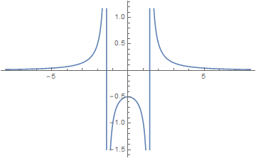
 with singularities at
  2
2Considering the sequence ![]() in
in ![]() shows that the actual limit
shows that the actual limit ![]() is not contained in
is not contained in ![]() .
.
![]()
Hence, a key question is:
- What condition on a sequence of numbers is necessary and sufficient for the sequence to converge to a limit but does not explicitly involve the limit?
If we already knew the limit in advance, the answer would be trivial. In general, however, the limit is not known and thus the question not easy to answer. It turns out that the Cauchy-property of a sequence is not only necessary but also sufficient. That is, every convergent Cauchy sequence is convergent (sufficient) and every convergent sequence is a Cauchy sequence (necessary).
Note that every Cauchy sequence is bounded. To see this set ![]() , then there is a
, then there is a ![]() :
: ![]() and thus
and thus ![]() for all
for all ![]() . This means that all points
. This means that all points ![]() with
with ![]() lies within a ball of radius 1 with
lies within a ball of radius 1 with ![]() as its center.
as its center.
Theorem 3.2 (Cauchy Sequences & Convergence):
In an Euclidean space ![]() every Cauchy sequence is convergent.
every Cauchy sequence is convergent.
Proof: Let ![]() be a Cauchy sequence in
be a Cauchy sequence in ![]() and let
and let ![]() be the range of the sequence. If
be the range of the sequence. If ![]() is finite, then all except a finite number of the terms
is finite, then all except a finite number of the terms ![]() are equal and hence
are equal and hence ![]() converges to this common value.
converges to this common value.
Now suppose ![]() is infinite. We use the Balzano-Weierstrass Theorem to show that
is infinite. We use the Balzano-Weierstrass Theorem to show that ![]() has an accumulation point
has an accumulation point ![]() , and then we show that
, and then we show that ![]() converges to
converges to ![]() . First, recall that each Cauchy sequence is bounded. Hence, since
. First, recall that each Cauchy sequence is bounded. Hence, since ![]() is infinite there must be an accumulation point
is infinite there must be an accumulation point ![]() according to the Bolzano-Weierstrass Theorem.
according to the Bolzano-Weierstrass Theorem.
Now let ![]() , then there exist a
, then there exist a ![]() such that
such that ![]() whenever
whenever ![]() . Hence, if
. Hence, if ![]() we have
we have
![]() ,
,
so ![]() .
.![]()
Let us furthermore connect the concepts of metric spaces and Cauchy sequences.
Definition 3.3: (Complete Metric Space & Banach Space)
A metric space ![]() is called complete (or a Cauchy space) if every Cauchy sequence of points in
is called complete (or a Cauchy space) if every Cauchy sequence of points in ![]() has a limit that is also in
has a limit that is also in ![]() .
.
A Banach space is a complete normed vector space, i.e. a real or complex vector space on which a norm is defined.
![]()
Complete and Banach space will become important in Functional Analysis, for instance.
One-Sided Limit of a Function
In this section it is about the limit of a sequence that is mapped via a function to a corresponding sequence of the range. As mentioned before, this concept is closely related to continuity. Let ![]() denote the standard metric space on the real line with
denote the standard metric space on the real line with ![]() and
and ![]() .
.
Consider the Heaviside function as shown below. In the one-dimensional metric space ![]() there are only two ways to approach a certain point
there are only two ways to approach a certain point ![]() on the real line. For instance, the point
on the real line. For instance, the point ![]() can be either be approached from the negative (denoted by
can be either be approached from the negative (denoted by ![]() ) or from the positive (denoted by
) or from the positive (denoted by ![]() ) part of the real line. Sometimes this is stated as the limit
) part of the real line. Sometimes this is stated as the limit ![]() is approached “from the left/righ” or “from below/above”.
is approached “from the left/righ” or “from below/above”.
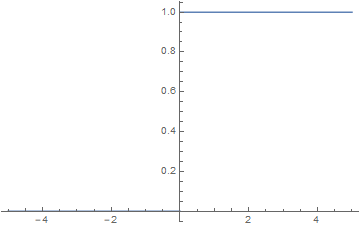
The Heaviside function does not have a limit at ![]() , because if you approach 0 from positive numbers the value is 1 while if you approach from negative numbers the value is 0. As we know, the limit needs to be unique if it exists.
, because if you approach 0 from positive numbers the value is 1 while if you approach from negative numbers the value is 0. As we know, the limit needs to be unique if it exists.
Hence, by writing the left-sided limit
(6) ![]()
we mean that for every real number ![]() , there is a
, there is a ![]() , such that
, such that
(7) ![]()
Left-sided means that the ![]() -value increases on the real axis and approaches from the left to the limit point
-value increases on the real axis and approaches from the left to the limit point ![]() . Hence,
. Hence, ![]() is positive.
is positive.
Accordingly, by writing the right-sided limit
(8) ![]()
we mean that for every real number ![]() , there is a
, there is a ![]() , such that
, such that
(9) ![]()
Right-sided means that the ![]() -value decreases on the real axis and approaches from the right to the limit point
-value decreases on the real axis and approaches from the right to the limit point ![]() . Hence,
. Hence, ![]() is positive.
is positive.
![]()
Consider that the left-sided and right-sided limits are just the restricted functions, where the domain is constrained to the “right-hand side” or “left-hand side” of the domain relative to its limit point ![]() .
.
That is, for ![]() being the metric space the left-sided and the right-sided domains are
being the metric space the left-sided and the right-sided domains are ![]() and
and ![]() , respectively. If we then consider the limit of the restricted functions
, respectively. If we then consider the limit of the restricted functions ![]() and
and ![]() , we get an equivalent to the definitions above.
, we get an equivalent to the definitions above.
Having said that, it is clear that all the rules and principles also apply to this type of convergence. In particular, this type will be of interest in the context of continuity.
Literature:
[1]
[2]
[3]


